Spherical varieties
The right-hand side of the Theorem is built from \(X\) alone: a torus \(\AXs\), a translate by \(\dXh\), a finite group \(\WX\). All three are read off one piece of geometry, the open orbit of a Borel subgroup. The four examples set up here recur on every later page.
SettingWhat is fixed once and for all?
\(F\) is a non-archimedean local field with ring of integers \(\cO\), uniformizer \(\vpi\) and residue field \(\Fq\); \(\val:F^\times\to\Z\) is the valuation with \(\val\vpi=1\), and \(|x|=q^{-\val x}\). \(G\) is a split connected reductive group over \(\cO\) with a Borel subgroup \(B\) and a split maximal torus \(T\subseteq B\); \(N\) is the unipotent radical of \(B\). The maximal compact subgroup is
\[K:=G(\cO).\]\(X\) is a \(G\)-scheme over \(\cO\); \(G\) acts on the left, \(g\cdot x\). Its \(F\)-points \(X(F)\) carry the action of \(G(F)\) and its integral points \(X(\cO)\subseteq X(F)\) are stable under \(K\). Sakellaridis writes \(H\backslash G\) with a right action; the dictionary is on the Theorem page.
Throughout, the examples are over \(G=\GL_n\) or products of such; then \(B\) is the upper triangular matrices, \(T\) the diagonal ones, and \(K=\GL_n(\cO)\).
Spherical varietiesWhat makes \(K\backslash X(F)\) small enough to be indexed by a lattice?
(spherical variety) [SV, §1.1] Definition
A normal \(G\)-variety \(X\) is spherical if a \(B\) has an open orbit \(\Xo\subseteq X\). Since \(\Xo\) is a single \(B\)-orbit,
\[\dim X=\dim\Xo\le\dim B .\]Why \(K\)-orbits are few: by the Iwasawa decomposition \(G(F)=B(F)K\), a \(K\)-orbit meets the open \(B\)-orbit in a set that \(B(F)\) moves around, and \(B(F)/B(\cO)\) is a lattice of translations \(\LT\) times a compact piece. The lattice that survives is the subject of the next page.
The four running examples, each with the open \(B\)-orbit written out:
(\(\GL_2/\SL_2\simeq\Gm\))
\(G=\GL_2\) acts on \(X=\Gm\) through the determinant, \(g\cdot x=\det(g)\,x\). The stabilizer of \(1\) is \(\SL_2\), so \(X=\GL_2/\SL_2\). \(B\) already acts transitively (\(\det B=\Gm\)), so \(\Xo=X\); \(\dim X=1\le3=\dim B\).
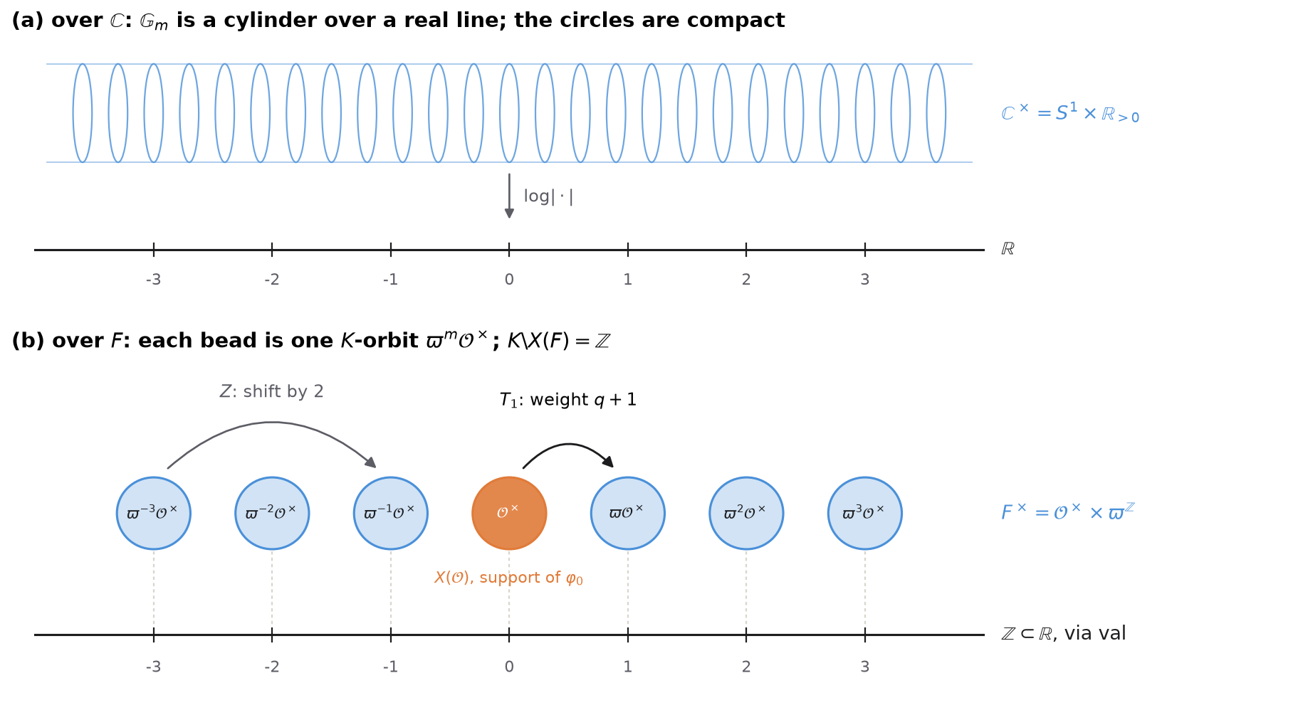
How the literature pictures \(\GL_2/\SL_2\simeq\Gm\)
The figure above is the picture behind three standard ones, each drawn for a different invariant:
- The building of the torus (Bruhat–Tits). For a split torus \(A\), the apartment is \(\Lambda_A\otimes\R\), and \(A(F)\) acts on it by translation through \(\val\). For \(\Gm\) it is exactly the line of panel (b), and the beads are \(\Gm(F)/\Gm(\cO)=\Z\) inside it. The tree of \(\PGL_2\) is built from such lines (apartments).
- The valuation cone (Luna–Vust, Knop; [SV, §2.1]). One draws \(\LX\otimes\Q\) and shades the cone \(\Vc\) of invariant valuations. For \(\Gm\), \(\LX=\Z\) and \(\Vc\) is the whole line, with no wall; for \(\GL_2/T\) it is a half-line. See panel (a) against (b) of the cone figure on the torus page.
- The dual torus (Satake, Sakellaridis). One draws the real points \((\log_q|x_1|,\log_q|x_2|)\) of \(\As\). For \(\Gm\), \(\AXs\) is the diagonal \(\{(y,y)\}\), and \(\dXh\) moves it off the mirror of \(W\) (A* and A_X*). The line of panel (b) and this line are dual: \(\one_{\vpi^m\cO^\times}\mapsto y^m\).
(\(\GL_2/T\), pairs of lines)
\(G=\GL_2\) acts on ordered pairs of distinct lines in the plane,
\[X=\{(\ell_1,\ell_2)\in\mathbb P^1\times\mathbb P^1:\ \ell_1\ne\ell_2\},\qquad\Stab(F e_1,F e_2)=T,\qquad X=\GL_2/T .\]Write a line other than \(\infty:=F e_1\) as \([x:1]\). \(B\) fixes \(\infty\) and acts on the other lines by \(x\mapsto(ax+b)/d\); these affine maps move any two distinct points to any other two, so
\[\Xo=\{(\ell_1,\ell_2):\ \ell_1\ne\infty\ne\ell_2\},\qquad\dim X=2\le3 .\](the group \(\GL_2\) under \(\GL_2\times\GL_2\))
\(G=\GL_2\times\GL_2\) acts on \(X=\GL_2\) by \((g_1,g_2)\cdot x=g_1xg_2^{-1}\); the stabilizer of \(1\) is the diagonal. Take the Borel subgroup \(B\times B^-\) (\(B^-\) lower triangular). The orbit of \(1\) is \(BB^-\), the matrices with an “upper times lower” factorization, which are exactly those with \(x_{22}\ne0\):
\[\Xo=\{x\in\GL_2:\ x_{22}\ne0\},\qquad\dim X=4\le6 .\](\(\Aff^n\) under \(\GL_n\))
\(G=\GL_n\) acts on column vectors \(X=\Aff^n\). For \(b\in B\), \(be_n\) is the last column of \(b\), whose last entry is a unit; so
\[\Xo=B\cdot e_n=\{v:\ v_n\ne0\},\qquad\dim X=n\le\tfrac{n(n+1)}2 .\]This example has its own tab, 𝔸ⁿ under GLₙ.
Two non-examples:\(\GL_2\) acting on \(\Aff^2\times\Aff^2\) (pairs of vectors: \(\dim 4>3\)) is not spherical; \(\GL_3/T\) is not spherical either (\(\dim6=\dim B\), but the generic \(B\)-stabilizer is the centre, of dimension \(1\), so \(B\)-orbits have dimension \(5\)).
Homogeneous, affine, quasi-affineWhich spherical varieties does the Theorem cover?
Definition
\(X\) is homogeneous if \(G\) acts transitively on \(X(\bar F)\), i.e. \(X=G/H\) for the stabilizer \(H\) of a point; it is affine if it is an affine variety, and quasi-affine if it is open in an affine variety.
(Matsushima's criterion) [Matsushima] Proved (cited)
For \(H\subseteq G\) closed, \(G/H\) is affine if and only if \(H\) is reductive.
So the hypothesis “homogeneous affine” of the Theorem means \(X=G/H\) with \(H\) reductive. Sakellaridis–Venkatesh work with homogeneous quasi-affine \(X\); the variety \(\Aff^n\) is in neither class.
| \(X\) | \(H\) | homogeneous | affine |
|---|---|---|---|
| \(\GL_2/\SL_2\simeq\Gm\) | \(\SL_2\) | yes | yes |
| \(\GL_2/T\) | \(T\) | yes | yes |
| \(\GL_2\) under \(\GL_2^2\) | diagonal \(\GL_2\) | yes | yes |
| \(\Aff^n\smallsetminus\{0\}\) | \(\Stab(e_n)\) | yes | no, quasi-affine (\(n\ge2\)) |
| \(\Aff^n\) | — | no: orbits \(\{0\}\), \(\Aff^n\smallsetminus\{0\}\) | yes |
For \(n\ge2\), \(\Stab(e_n)=\{g:\ ge_n=e_n\}\) contains the lower unitriangular matrices, a maximal unipotent subgroup, so it is not reductive; \(\Aff^n\smallsetminus\{0\}\) is the open \(G\)-orbit of \(\Aff^n\), written \(\Xb\) on the 𝔸ⁿ pages.
A non-homogeneous \(X\) is harder because \(\CK\) is no longer spanned by indicators of \(K\)-orbits: \(\{0\}\) is a \(K\)-orbit that is not open, and a Schwartz function only has to be constant near \(0\). The fix, a lattice basis instead of an orbit basis, is on 𝔸ⁿ: spherical level.
The parabolic \(\PX\) and the Levi \(\LevX\)Which part of \(G\) does not see the open orbit at all?
(associated parabolic) [Sak, §2.1, p. 8; SV, §2.1] Definition
The parabolic of \(X\) is the stabilizer of the open \(B\)-orbit, and \(\LevX\) is a Levi subgroup of it containing \(T\), chosen as in [Sak, §2.1] (for a symmetric variety, the \(\theta\)-stable Levi subgroup of a minimal \(\theta\)-split parabolic):
\[\PX:=\{g\in G:\ g\Xo=\Xo\}\supseteq B,\qquad T\subseteq\LevX\subseteq\PX .\]Fix a base point \(x_0\in\Xo(\cO)\) and let \(H\) be its stabilizer.
The semisimple part of \(\LevX\) fixes \(x_0\); only the torus \(\LevX/[\LevX,\LevX]\) moves it. That torus, cut down by \(H\), is \(\AX\) (next page), and the half-sum of positive roots of \(\LevX\) gives \(\dX\) (δ(X)).
| \(X\) | \(\PX\) | \(\LevX\) | reason |
|---|---|---|---|
| \(\GL_2/\SL_2\) | \(\GL_2\) | \(\GL_2\) | \(\Xo=X\) |
| \(\GL_2/T\) | \(B\) | \(T\) | \(g\Xo=\Xo\) iff \(g\infty=\infty\) |
| \(\GL_2\) under \(\GL_2^2\) | \(B\times B^-\) | \(T\times T\) | \(g_1BB^-g_2^{-1}=BB^-\) iff \(g_1\in B\), \(g_2\in B^-\) |
| \(\Aff^n\) | \(P_{n-1,1}\) | \(\GL_{n-1}\times\GL_1\) | last row of \(g\) must be \((0,\dots,0,*)\) |
| \(\GL_4/\Sp_4\) | \(P_{2,2}\) | \(\GL_2\times\GL_2\) | [Sak, Appendix A, row 2] |
How the rows are computed
\(\GL_2/T\): \(\Xo\) is “neither line is \(\infty\)”; \(g\) preserves this set iff \(g\) fixes \(\infty=Fe_1\), i.e. \(g\in B\). Then \(\LevX=T\) and \([T,T]=1\subseteq H\) trivially.
\(\Aff^n\): \(g\) preserves \(\{v_n\ne0\}\) iff the \(n\)-th coordinate of \(gv\) is a nonzero multiple of \(v_n\), i.e. the last row of \(g\) is \((0,\dots,0,c)\). The block-diagonal Levi is \(\GL_{n-1}\times\GL_1\), and \([\LevX,\LevX]=\SL_{n-1}\) fixes \(x_0=e_n\), as the Lemma predicts.
The group: \(\LevX=T\times T\), and \(\LevX\cap H\) is the diagonal \(T\).
ColoursWhat is the complement of the open orbit made of?
[SV, §2.3.7] Definition
A colour of \(X\) is a \(B\)-stable prime divisor of \(X\) that is not \(G\)-stable.
| \(X\) | colours | \(G\)-stable divisors |
|---|---|---|
| \(\GL_2/\SL_2\) | none | none |
| \(\GL_2/T\) | \(\{\ell_1=\infty\}\), \(\{\ell_2=\infty\}\) | none |
| \(\GL_2\) under \(\GL_2^2\) | \(\{x_{22}=0\}\) | none |
| \(\Aff^n\), \(n\ge2\) | \(\{v_n=0\}\) | none (\(\{0\}\) has codimension \(n\)) |
| \(\Aff^1\) under \(\GL_1\) | none | \(\{0\}\) |
Colours enter in two places later: the colour of \(\Aff^n\) points towards the extra orbit \(\{0\}\) (𝔸ⁿ geometry), and Sakellaridis's L-value formula is indexed by colour valuations ([Sak, §7.1]; hypothesis (A4)).
Where this goes
| page | object | built from |
|---|---|---|
| A_X and the cone | \(\AX\), \(\LX\), \(\LXp\) | \(\LevX/(\LevX\cap H)\); invariant valuations |
| K- and I-orbits | \(K\backslash X(F)\simeq\LXp\) | points \(\lambda(\vpi)x_0\) |
| A* and A_X* | \(\As\), \(\AXs\subseteq\As\) | \(T\twoheadrightarrow\AX\) |
| δ(X) | \(\dXh\in\As\) | positive roots of \(\LevX\) |
| W_X | \(\WX\) | reflections fixing the cone |