Geometry · 4

\(K\)- and \(I\)-orbits on \(X(F)\)

\(\CK\) is a space of functions on \(K\backslash X(F)\). For the varieties of the Theorem it is \(\LXp\), the monoid of the previous page. This page proves that by hand in three examples, shows two ways it can fail, and refines \(K\)-orbits to Iwahori orbits for the Iwahori tab.

Sections · arrows: “is used by”

Orbits and the space \(\CK\)When is \(\CK\) spanned by indicators of \(K\)-orbits?

\(\Sw(X):=C_c^\infty(X(F))\) is the space of locally constant, compactly supported functions \(X(F)\to\C\), and \(\CK:=\Sw(X)^K\).

(orbits and the basis of \(\CK\)) Proved here

Every \(K\)-orbit in \(X(F)\) is compact. If \(X=G/H\) is homogeneous and \(\operatorname{char}F=0\), every \(K\)-orbit is also open, and

\[\CK=\bigoplus_{Kx\in K\backslash X(F)}\C\,\one_{Kx}\qquad\text{(finite sums).}\]

Proof

\(Kx\) is the image of the compact group \(K\) under \(k\mapsto kx\).
For homogeneous \(X\), \(X(F)\) is a finite union of \(G(F)\)-orbits, indexed by \(\ker\big(H^1(F,H)\to H^1(F,G)\big)\), which is finite for \(\operatorname{char}F=0\) [Serre, Galois cohomology, III.4.3]. Each \(G(F)\)-orbit is open: the orbit map \(G\to X\) is smooth, so \(G(F)\to G(F)x\) is a submersion of \(p\)-adic manifolds and hence open, and \(Kx\) is the image of the open set \(K\).
A \(K\)-invariant function is constant on each \(K\)-orbit; a compactly supported one meets finitely many of these open orbits.

For \(\Aff^n\) the orbit \(\{0\}\) is not open, and \(\one_{\cO^n}\) is not a finite sum of orbit indicators: the Lemma's second half needs homogeneity (last section). The characteristic-\(0\) input in step 2 is one of the places discussed on Characteristic 0?.

The generalized Cartan decompositionWhy are \(K\)-orbits labelled by valuations?

Recall the points \(x_\lambda=\tilde\lambda(\vpi)x_0\), \(\lambda\in\LX\), from the torus page.

(generalized Cartan decomposition) [Sak, Axiom 2.4.1 and §8; SV, Thm. 5.3.3] Proved (cited), under hypotheses

Under Sakellaridis's hypotheses (A1)–(A5) (Hypotheses),

\[K\backslash X(F)\xrightarrow{\ \sim\ }\LXp,\qquad Kx_\lambda\longleftarrow\!\shortmid\ \lambda .\]

Axiom 2.4.1 says that the points \(x_\lambda\), \(\lambda\in\LXp\), meet every \(K\)-orbit and that distinct \(\lambda\) give distinct orbits; under (A5) this becomes the bijection above [Sak, §8, p. 63]. Sakellaridis does not prove the axiom in general: it is proved over \(\C[\![t]\!]\) by Luna–Vust, at almost every place of a global field in [Sak12, Thm. 2.3.8] following Gaitsgory–Nadler, and for symmetric varieties by Delorme–Sécherre and Benoist–Oh ([Sak, §2.4]; [SV, Thm. 5.3.3]). The three running examples, by hand:

(\(\GL_2/\SL_2\))

\(X(F)=F^\times\) and \(K\) acts through \(\det K=\cO^\times\), so

\[K\backslash X(F)=F^\times/\cO^\times=\{\vpi^m\cO^\times\}_{m\in\Z}\simeq\Z=\LXp,\qquad x_m=\vpi^m,\qquad X(\cO)=\cO^\times .\]

The orbits are the beads of the figure 𝔾ₘ as a line.

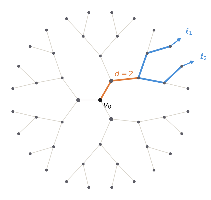
(\(\GL_2/T\): two ends of the tree)

A line \(\ell\in\mathbb P^1(F)=\mathbb P^1(\cO)\) is spanned by a primitive vector \(u\in\cO^2\) (one coordinate a unit), unique up to \(\cO^\times\). For a pair of distinct lines put

\[d(\ell_1,\ell_2):=\val\det(u_1\,|\,u_2)\in\Z_{\ge0}.\]

Then \(K\backslash X(F)\simeq\Z_{\ge0}=\LXp\) via \(d\), with \(x_d=\diag(\vpi^d,1)\cdot x_0\) for \(x_0=(F e_2,\,F(e_1+e_2))\), and \(X(\cO)=\{d=0\}\): the pairs whose reductions mod \(\vpi\) are distinct.

Proof

\(d\) is well defined (units change \(\det\) by units) and \(K\)-invariant (\(\det k\in\cO^\times\)).
\(K\) is transitive on \(\mathbb P^1(F)\) (a primitive vector extends to a basis of \(\cO^2\)), so take \(\ell_1=Fe_2\). Its stabilizer in \(K\) is \(B^-(\cO)\), which acts on the remaining lines \([1:y]\) by \(y\mapsto(c+dy)/a\), \(a,d\in\cO^\times\), \(c\in\cO\). The orbits are \(\{y\in\cO\}\) and \(\{\val y=-d\}\) for each \(d\ge1\).
For \(y\in\cO\), \(\det\big((0,1)^{\mathsf T}\,|\,(1,y)^{\mathsf T}\big)=-1\), so \(d=0\); for \(\val y=-d\), the primitive vector is \((\vpi^d,\vpi^dy)\) and \(d(\ell_1,\ell_2)=d\). So \(d\) separates the orbits and takes every value \(\ge0\).
\(\diag(\vpi^d,1)\) sends \(x_0\) to \((Fe_2,F(\vpi^de_1+e_2))\), with \(\det=-\vpi^d\). For \(\lambda=-d\lt0\) it gives \((Fe_2,F(e_1+\vpi^de_2))\) with \(d=0\): negative labels land in the orbit of \(0\), which is why only \(\LXp\) indexes orbits.

A radial tree of valence 3 around a base vertex v0; two boundary rays labelled l1 and l2 joined by a blue geodesic; the orange path from v0 to that geodesic has two edges, labelled d = 2. — \(q=2\): the lines \(\ell_1,\ell_2\) are ends of the tree of \(\PGL_2(F)\), and \(d(\ell_1,\ell_2)\) is the distance (orange) from the vertex \(v_0=[\cO^2]\) to the geodesic joining them (blue) [Serre, Trees, II.1].

(the group: the classical Cartan decomposition)

\[\GL_2(F)=\bigsqcup_{\lambda_1\ge\lambda_2}K\,t^\lambda K,\qquad t^\lambda=\diag(\vpi^{\lambda_1},\vpi^{\lambda_2}),\]

by elementary divisors (Smith normal form over \(\cO\)). So \(K\backslash X(F)\) for \(X=\GL_2\) under \(\GL_2^2\) is \(\{\lambda_1\ge\lambda_2\}=\LXp\), and \(X(\cO)=\GL_2(\cO)=Kt^0K\).

When the bijection failsWhat extra orbits can a local field create?

Sakellaridis's remark after Axiom 2.4.2 [Sak, p. 11] gives two failures, both with a disconnected \(H\):

\(X=\{\pm1\}\backslash\Gm\) under \(\Gm\): the \(K\)-orbits on \(X(F)\simeq F^\times\) are the classes of \(F^\times/\cO^{\times2}\), two above each valuation when \(p\) is odd, while \(\LXp=\Z\);
\(X=\Orth_2\backslash\GL_2\), the nondegenerate quadratic forms in two variables: four points of \(\AX(\cO)/T(\cO)\) fall into only two \(K\)-orbits, so distinct representatives can lie in one \(K\)-orbit.

He adds: “We certainly expect that the second map is bijective when \(H\) is connected.” The same square classes make \(\SL_2/T\) fail; there they break spherical generation itself (hypothesis (A5)).

Iwahori orbitsHow does a \(K\)-orbit split under the smaller group \(I\)?

The is \(I:=\{k\in K:\ k\bmod\vpi\in B(\Fq)\}\). Sakellaridis's Axiom 2.4.2 asks \(Ix_\lambda\subseteq B(\cO)x_\lambda\) for \(\lambda\in\LXp\) [Sak, p. 11]; it is what lets him compute \(I\)-invariant vectors first and average to \(K\) afterwards (the Casselman–Shalika method, [Sak, §1.2]). The \(I\)-orbits are what \(\CI=\Sw(X)^I\) is spanned by, and they are used on the Iwahori tab. Two examples:

(\(\mathbb P^1\))

\(K\) is transitive on \(\mathbb P^1(F)\); reduction mod \(\vpi\) is \(I\)-equivariant onto the action of \(B(\Fq)\) on \(\mathbb P^1(\Fq)\), which has the two orbits \(\{\infty\}\) and \(\Aff^1(\Fq)\). So

\[I\backslash\mathbb P^1(F)=\{U_1,U_2\},\qquad U_1=\{[1:y]:\ y\in\vpi\cO\},\quad U_2=\{[x:1]:\ x\in\cO\}.\]

(\(\Aff^n\))

Each shell \(X_m=\{\ord v=m\}\) (\(\ord v=\min_i\val v_i\)) is one \(K\)-orbit and splits into \(n\) \(I\)-orbits, according to the last index at which the minimum is attained; the pictures are on 𝔸ⁿ geometry.

Non-homogeneous \(X\)What replaces the orbit basis when an orbit is not open?

For \(X=\Aff^n\), the \(K\)-orbits are the shells \(X_m\), \(m\in\Z\), and the point \(\{0\}\). The shells are the \(K\)-orbits of the open orbit \(\Xb\), labelled by \(\LXp=\Z\) of \(\Xb\). A function in \(\CK\) is constant on each shell, vanishes on \(X_m\) for \(m\ll0\), and is constant on a neighbourhood \(\vpi^N\cO^n\) of \(0\). So the indicators of the lattices form a basis:

\[\CK=\bigoplus_{m\in\Z}\C\,\one_{\vpi^m\cO^n},\qquad\one_{X_m}=\one_{\vpi^m\cO^n}-\one_{\vpi^{m+1}\cO^n}.\]

The orbit indicators \(\one_{X_m}\) span only the hyperplane of functions vanishing at \(0\). This is the first difference with the Theorem's setting; the second (no invariant measure on \(\Xb\)) is on 𝔸ⁿ: spherical level.