Archived 2026-10-20 — the maintained version is the 𝔸ⁿ pages of the basic-function site (geometry, orbits and lattices there; generation, the origin, the sheaf sketch and the paper on its Iwahori page). This copy is kept unchanged for the links of earlier runs.
Conventions, the criterion \(\mathcal H_I\cdot\varphi_0=C_I\iff(\mathcal H_K\cdot\varphi_0=C_K\text{ and }\mathcal H_I\cdot C_K=C_I)\), the obstruction modules and the Steinberg examples: Iwahori pages. Tools and sweeps: F1; the other families: F2. Column vectors, \(G\) acting on the left, left \(\mathcal H_I\)-modules; the pasted rank-one note (its Theorem 4, row vectors and right modules) is the case \(n=2\) of Theorem 3 below after transposing.
1 · Setting and the valuation picture
\(G=\mathrm{GL}_n\supseteq B\) upper triangular, \(X=\mathbb A^n\) with \(g\cdot v=gv\) on column vectors. \(X\) is spherical (\(B\) has an open orbit), and the stabilizer in \(B\) of a point of that orbit is a connected algebraic group:
$$\begin{gathered}B\cdot e_n=\{v:\ v_n\ne0\}\ \text{ is open and dense},\\[6pt]\operatorname{Stab}_B(e_n)=\{b\in B:\ b_{in}=0\ (i<n),\ b_{nn}=1\}\ \text{ is connected},\end{gathered}$$so \(X\) lies in the paper's class (smooth affine spherical, connected \(B\)-stabilizers; 7). \(F\) is non-archimedean with ring of integers \(\mathcal O\), uniformizer \(t\) and residue field \(\mathbb F_q\); in every example and picture \(F=k(\!(t)\!)\) and \(\mathcal O=k[[t]]\) with \(k=\mathbb F_q\); then \(\operatorname{val}\) is the order of vanishing at \(t\), and
$$\begin{gathered}X(F)=F^n,\qquad X(\mathcal O)=\mathcal O^n,\qquad\varphi_0=\mathbf 1_{\mathcal O^n},\\[6pt]K=\mathrm{GL}_n(\mathcal O),\qquad I=\{k\in K:\ k\bmod t\in B(\mathbb F_q)\},\qquad K_1=1+tM_n(\mathcal O)\subseteq I .\end{gathered}$$The valuation-plane pictures are for \(n=2\) (Figure 3 also offers a coordinate view for larger \(n\)), in valuation coordinates: a nonzero \(v=(v_1,v_2)\) is drawn at \((a,b)=(\operatorname{val}v_1,\operatorname{val}v_2)\), a zero coordinate at \(\infty\). One point of the plane stands for every vector with those two valuations.
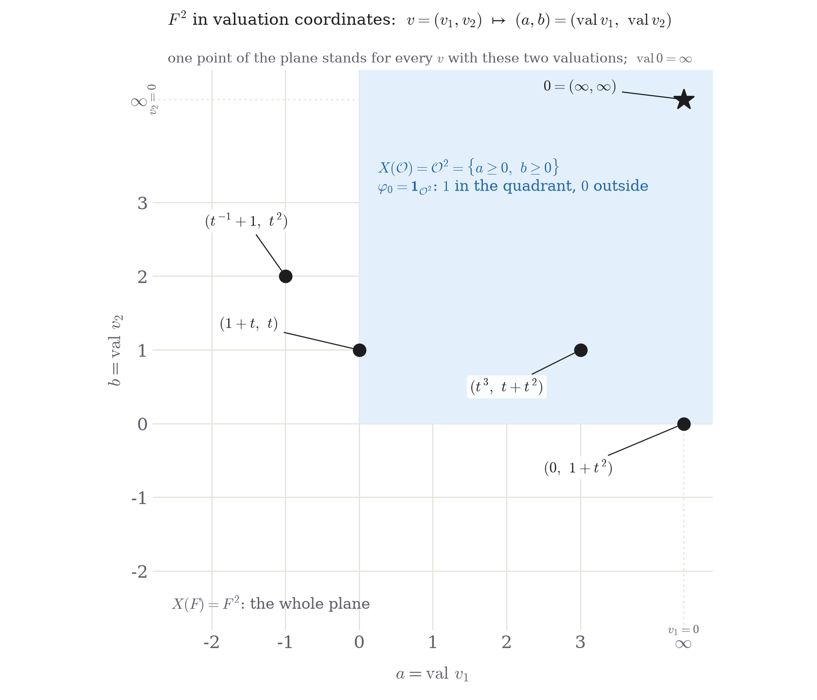
Definition (order and last coordinate). For \(v\in F^n\setminus0\) write \(\operatorname{val}v=(\operatorname{val}v_1,\dots,\operatorname{val}v_n)\in(\mathbb Z\cup\{\infty\})^n\). The order of \(v\) is the smallest valuation of a coordinate, and \(\operatorname{last}v\) is the last index at which that minimum is attained:
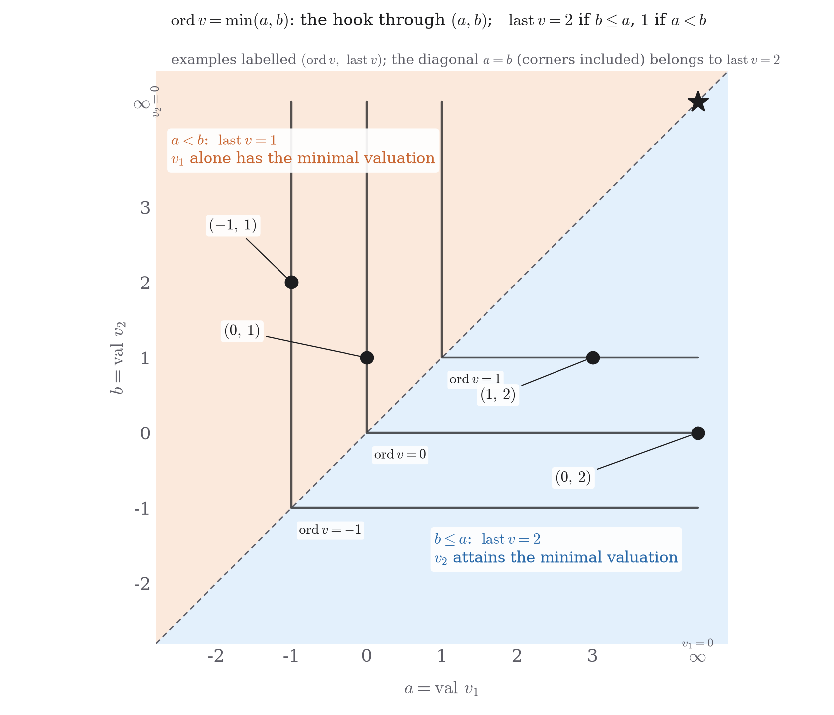
$$\operatorname{ord}v:=\min_i\operatorname{val}v_i\in\mathbb Z,\qquad\operatorname{last}v:=\max\{i:\ \operatorname{val}v_i=\operatorname{ord}v\}\in\{1,\dots,n\}.$$In words. Equivalently \(\operatorname{ord}v\) is the largest \(m\) with \(v\in t^m\mathcal O^n\), so \(v=t^{\operatorname{ord}v}v_0\) with \(v_0\) primitive (some coordinate a unit), and \(\operatorname{last}v\) is the position of the last nonzero coordinate of \(v_0\bmod t\in\mathbb F_q^n\). The order says at which scale \(v\) lives; the last coordinate says which basis direction carries its leading term, counted from the end, which is exactly what an upper triangular matrix cannot change.
Definition (primitive vector). A vector \(u\in\mathcal O^n\) is primitive if any of the following equivalent conditions holds:
$$u\notin t\mathcal O^n\quad\Longleftrightarrow\quad \operatorname{ord}u=0\quad\Longleftrightarrow\quad u\bmod t\ne0\quad\Longleftrightarrow\quad \exists i:\ u_i\in\mathcal O^\times.$$For \(n=2\), this is \(u=(x,y)\in\mathcal O^2\) with \(x\) or \(y\) a unit: \((1+t,t)\), \((t,1+t)\) and \((1,1)\) are primitive; \((t,t^2)\) and \((0,0)\) are not.
Example (\(n=2\)). For \(v=(v_1,v_2)\) at \((a,b)\): \(\operatorname{ord}v=\min(a,b)\), so the vectors of order \(m\) fill the hook \(\{\min(a,b)=m\}\), the L-shape made of the rays \(b=m,\ a\ge m\) and \(a=m,\ b\ge m\) with corner \((m,m)\); \(\operatorname{last}v=2\) if \(b\le a\) (the minimum is attained at the second coordinate, possibly at both) and \(\operatorname{last}v=1\) if \(a<b\).
| \(v\) | \((a,b)\) | \(\operatorname{ord}v=\min(a,b)\) | \(v=t^{\operatorname{ord}v}v_0\) | \(v_0\bmod t\) | \(\operatorname{last}v\) |
|---|---|---|---|---|---|
| \((t^{-1}+1,\ t^2)\) | \((-1,2)\) | \(-1\) | \(t^{-1}(1+t,\ t^3)\) | \((1,0)\) | \(1\) |
| \((1+t,\ t)\) | \((0,1)\) | \(0\) | \((1+t,\ t)\) | \((1,0)\) | \(1\) |
| \((t,\ 1+t)\) | \((1,0)\) | \(0\) | \((t,\ 1+t)\) | \((0,1)\) | \(2\) |
| \((0,\ 1+t^2)\) | \((\infty,0)\) | \(0\) | \((0,\ 1+t^2)\) | \((0,1)\) | \(2\) |
| \((t^3,\ t+t^2)\) | \((3,1)\) | \(1\) | \(t\,(t^2,\ 1+t)\) | \((0,1)\) | \(2\) |
| \((t^2,\ t^2+t^3)\) | \((2,2)\) | \(2\) | \(t^2(1,\ 1+t)\) | \((1,1)\) | \(2\) |
Primitive vectors: four separate propositions
Proposition P1 (basis extension). Every primitive \(u\in\mathcal O^n\) extends to an \(\mathcal O\)-basis; equivalently, some \(k\in K\) satisfies \(ke_n=u\).
Proof
Proof, with explicit matrices for \(n=2\)
Choose a unit coordinate \(u_i\) and let \(k=(e_1|\cdots|\widehat{e_i}|\cdots|e_n|u)\in M_n(\mathcal O)\). Row \(i\) of \(k\) is zero except for \(u_i\) in column \(n\), so expanding along row \(i\),
$$\det k=(-1)^{i+n}\,u_i\cdot\det(\text{$k$ without row $i$ and column $n$})=(-1)^{i+n}\,u_i\det\mathbf 1_{n-1}=\pm u_i\in\mathcal O^\times,$$since deleting row \(i\) from the columns \(e_j\) (\(j\ne i\)) leaves the identity. Hence \(k\in\mathrm{GL}_n(\mathcal O)=K\), and \(ke_n=u\).
$$n=2:\qquad k=\begin{cases}\begin{pmatrix}1&x\\0&y\end{pmatrix},&y\in\mathcal O^\times,\\[8pt]\begin{pmatrix}0&x\\1&y\end{pmatrix},&x\in\mathcal O^\times;\end{cases}\qquad ke_2=(x,y).$$Proposition P2 (normalization and transitivity). Every \(v\ne0\) has a unique expression \(v=t^mu\) with \(m=\operatorname{ord}v\) and \(u\) primitive, and
$$K\cdot e_n=\mathcal O^n\setminus t\mathcal O^n,\qquad K\cdot(t^me_n)=X_m=t^m(\mathcal O^n\setminus t\mathcal O^n).$$For \(n=2\), \(X_0=\{a,b\ge0:\min(a,b)=0\}\) is the primitive hook; \(v=(t^3,t+t^2)=t(t^2,1+t)\) lies on \(X_1\).
Proof
Divide by the smallest coordinate valuation, apply P1, and use that \(k\) and \(k^{-1}\) preserve each \(t^m\mathcal O^n\).
Proposition P3 (congruence fibres). For primitive \(u\), \(v=t^mu\), and \(K_1=1+tM_n(\mathcal O)\),
$$K_1\cdot v=v+t^{m+1}\mathcal O^n=r_m^{-1}(u\bmod t),\qquad r_m:X_m\longrightarrow\mathbb F_q^n\setminus\{0\},\quad r_m(v)=t^{-m}v\bmod t.$$For \(n=2\), \(u=(t,1+t)\) gives \(K_1u=t\mathcal O\times(1+t\mathcal O)\); \(u=(1,1)\) gives \((1+t\mathcal O)^2\).
Proof
For any \(w\in\mathcal O^n\), choose a unit \(u_i\) and take \(A\) with column \(i\) equal to \(wu_i^{-1}\) and all other columns zero; then \(Au=w\) and \((1+tA)v=v+t^{m+1}w\).
Proposition P4 (the last nonzero coordinate). The upper triangular group \(B(\mathbb F_q)\) has exactly \(n\) orbits on \(\mathbb F_q^n\setminus\{0\}\):
$$B(\mathbb F_q)e_j=\{w:\ w_j\ne0,\ w_i=0\ (i>j)\},\qquad 1\le j\le n.$$For \(n=2\): \(Be_2=\{(x,y):y\ne0\}\) and \(Be_1=\{(x,0):x\ne0\}\); their inverse images under \(r_m\) are \(O_{m,2}\) and \(O_{m,1}\).
Proof
The column \(be_j\) has precisely this shape; conversely choose its \(j\)-th column to be \(w\), and all other diagonal entries to be \(1\).
Definition (the chain of lattices). For \(m\in\mathbb Z\) and \(0\le j\le n\), \(\Lambda_{m,j}\) is the lattice of vectors whose first \(j\) coordinates have valuation at least \(m\) and whose last \(n-j\) coordinates have valuation at least \(m+1\):
$$\Lambda_{m,j}:=\{v\in F^n:\ \operatorname{val}v_i\ge m\ (i\le j),\ \ \operatorname{val}v_i\ge m+1\ (i>j)\}=g_{m,j}\mathcal O^n,\qquad g_{m,j}:=t^m\operatorname{diag}(\underbrace{1,\dots,1}_{j},\underbrace{t,\dots,t}_{n-j}).$$Lowering \(j\) by one adds the condition \(\operatorname{val}v_j\ge m+1\), so \(\Lambda_{m,j}\supset\Lambda_{m,j-1}\); the ends match up, \(\Lambda_{m,0}=t^{m+1}\mathcal O^n=\Lambda_{m+1,n}\); and \(t\Lambda_{m,j}=\Lambda_{m+1,j}\). So all of them form one decreasing chain, periodic under multiplication by \(t\):
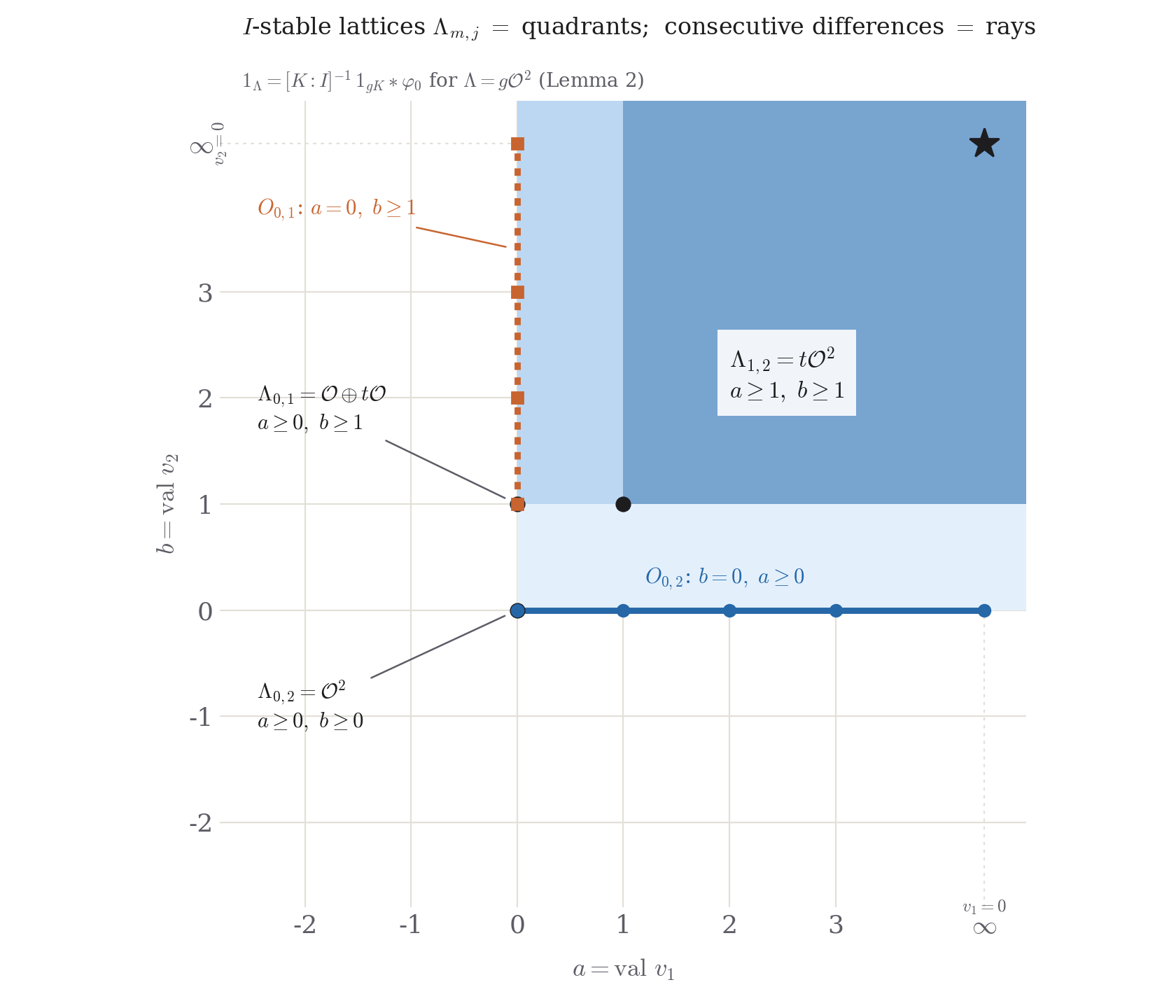
$$\cdots\supset\Lambda_{m,n}=t^m\mathcal O^n\supset\Lambda_{m,n-1}\supset\cdots\supset\Lambda_{m,1}\supset\Lambda_{m,0}=t^{m+1}\mathcal O^n=\Lambda_{m+1,n}\supset\Lambda_{m+1,n-1}\supset\cdots$$Intuition. Reduction \(v\mapsto t^{-m}v\bmod t\) identifies \(t^m\mathcal O^n/t^{m+1}\mathcal O^n\) with \(\mathbb F_q^n\), and \(\Lambda_{m,j}/t^{m+1}\mathcal O^n\) is the coordinate subspace \(\langle e_1,\dots,e_j\rangle\). So the chain inserts the standard flag \(0\subset\langle e_1\rangle\subset\langle e_1,e_2\rangle\subset\cdots\subset\mathbb F_q^n\) between \(t^{m+1}\mathcal O^n\) and \(t^m\mathcal O^n\), for every \(m\). This is where the two levels part: \(K\) preserves each \(t^m\mathcal O^n\) and acts on the quotient through all of \(\mathrm{GL}_n(\mathbb F_q)\), which moves the flag; \(I\) is the preimage of \(B(\mathbb F_q)\), the stabilizer of the standard flag, so \(I\) preserves every \(\Lambda_{m,j}\) (Lemma 1(c); by Lemma 2(c) there are no other \(I\)-stable lattices). Read \(j\) as the number of leading coordinates still allowed valuation exactly \(m\). Going down the chain tightens one coordinate at a time, from the last to the first, and what is lost at the step \(\Lambda_{m,j}\supset\Lambda_{m,j-1}\) are the vectors with \(\operatorname{val}v_j=m\) and all later coordinates deeper, i.e. those with \((\operatorname{ord}v,\operatorname{last}v)=(m,j)\). In the plane \(\Lambda_{m,j}\) is a quadrant, with corner \((m,m)\) for \(j=2\), \((m,m+1)\) for \(j=1\) and \((m+1,m+1)\) for \(j=0\): going down the chain moves the corner up one step, right one step, up, right, … along the diagonal, and each step removes one ray.
Example (\(n=2\)). Around \(\mathcal O^2\) the chain reads
$$\cdots\supset\Lambda_{-1,1}=t^{-1}\mathcal O\oplus\mathcal O\ \supset\ \Lambda_{0,2}=\mathcal O^2\ \supset\ \Lambda_{0,1}=\mathcal O\oplus t\mathcal O\ \supset\ \Lambda_{1,2}=t\mathcal O^2\ \supset\ \Lambda_{1,1}=t\mathcal O\oplus t^2\mathcal O\ \supset\cdots$$ $$g_{-1,1}=\begin{pmatrix}t^{-1}&0\\0&1\end{pmatrix},\qquad g_{0,2}=1,\qquad g_{0,1}=\begin{pmatrix}1&0\\0&t\end{pmatrix},\qquad g_{1,2}=t,\qquad g_{1,1}=\begin{pmatrix}t&0\\0&t^2\end{pmatrix},$$with corners \((-1,0)\), \((0,0)\), \((0,1)\), \((1,1)\), \((1,2)\). The index \(j=0\) only repeats a term: \(\Lambda_{-1,0}=\Lambda_{0,2}\) and \(\Lambda_{0,0}=\Lambda_{1,2}\). Each vector lies in an initial segment of the chain, and the last lattice containing it is \(\Lambda_{\operatorname{ord}v,\operatorname{last}v}\):
| \(v\) at \((a,b)\) | \(\Lambda_{-1,1}\): \(a\ge-1,\ b\ge0\) | \(\Lambda_{0,2}=\mathcal O^2\): \(a,b\ge0\) | \(\Lambda_{0,1}\): \(a\ge0,\ b\ge1\) | \(\Lambda_{1,2}=t\mathcal O^2\): \(a,b\ge1\) | \(\Lambda_{1,1}\): \(a\ge1,\ b\ge2\) | \((\operatorname{ord}v,\operatorname{last}v)\) |
|---|---|---|---|---|---|---|
| \((t^{-1}+1,\ t^2)\) at \((-1,2)\) | in | – | – | – | – | \((-1,1)\) |
| \((1+t,\ t)\) at \((0,1)\) | in | in | in | – | – | \((0,1)\) |
| \((t,\ 1+t)\) at \((1,0)\) | in | in | – | – | – | \((0,2)\) |
| \((0,\ 1+t^2)\) at \((\infty,0)\) | in | in | – | – | – | \((0,2)\) |
| \((t^3,\ t+t^2)\) at \((3,1)\) | in | in | in | in | – | \((1,2)\) |
Compare \((1+t,t)\) and \((t,1+t)\): the permutation matrix swaps them and lies in \(K\) but not in \(I\), and \(\Lambda_{0,1}\) contains the first but not the second. Figure 3 lets you move \(m\) and \(j\) and watch the quadrant, the next lattice and the ray between them.
Lemma 1 (orbits).
- The \(K\)-orbits on \(F^n\) are \(\{0\}\) and the shells \(X_m:=\{v:\ \operatorname{ord}v=m\}=t^m(\mathcal O^n\setminus t\mathcal O^n)\), \(m\in\mathbb Z\).
- The \(I\)-orbits on \(F^n\) are \(\{0\}\) and \(O_{m,j}:=\{v:\ \operatorname{ord}v=m,\ \operatorname{last}v=j\}\), \(m\in\mathbb Z\), \(1\le j\le n\); each shell is \(X_m=\bigsqcup_{j=1}^nO_{m,j}\).
- Every \(\Lambda_{m,j}\) is \(I\)-stable, and \(O_{m,j}=\Lambda_{m,j}\setminus\Lambda_{m,j-1}\). All orbits other than \(\{0\}\) are open and compact in \(F^n\); in the ind-scheme \(L\mathbb A^n\) (the sheaf picture, 6) \(\Lambda_{m,j}\) is the closure of \(O_{m,j}\).
Choose valuations above or click a grid point; the black ring marks the same vector in both panels.
(a) \(K\)-orbits
One hook per order; the selected hook is emphasized.
(b) \(I\)-orbits
Blue horizontal: last = 2. Orange vertical: last = 1.

Proof
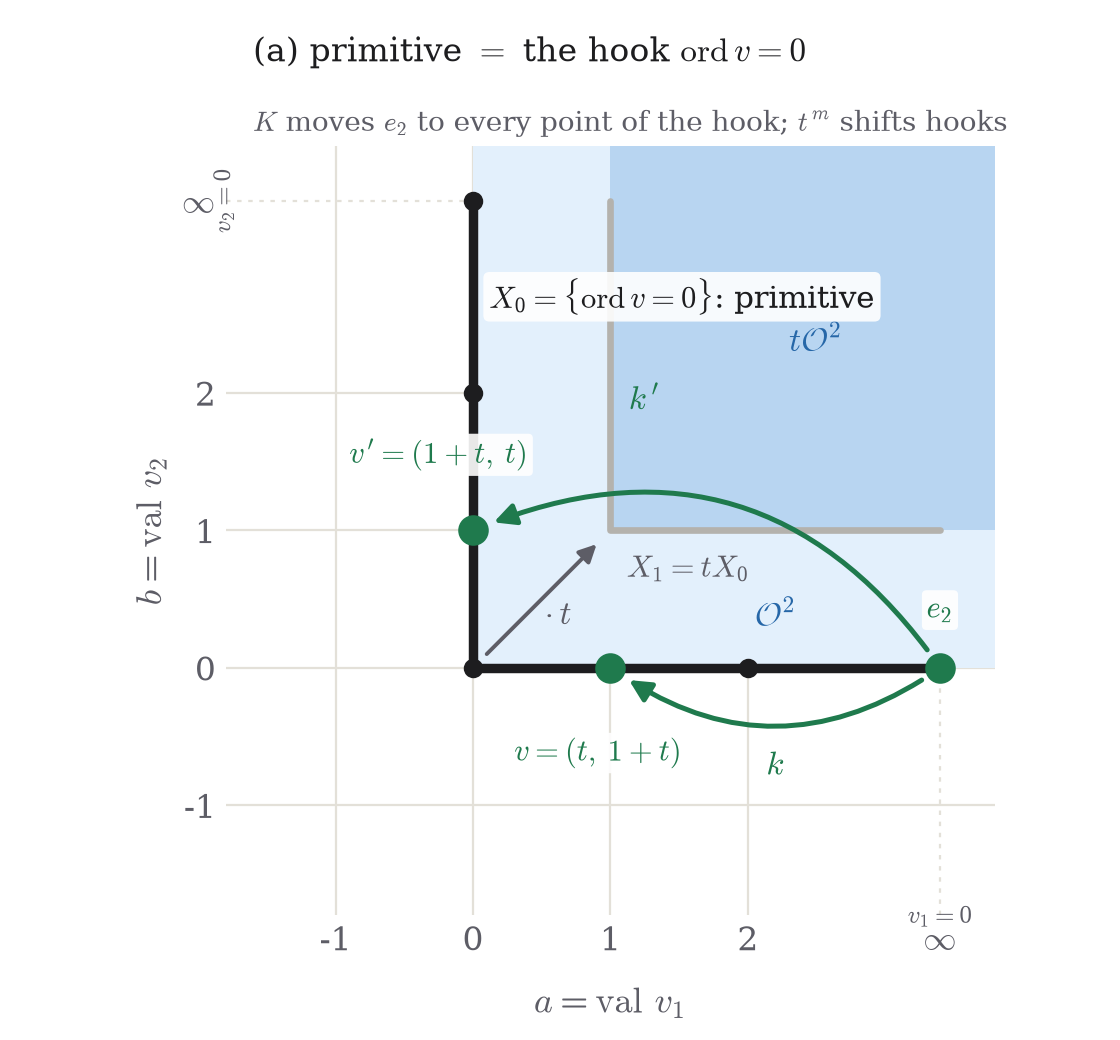
(a) Primitive vectors. P1 extends a primitive vector to a basis; P2 gives \(K\cdot v=X_m\). The two matrices in the picture realize P1 for \(n=2\).
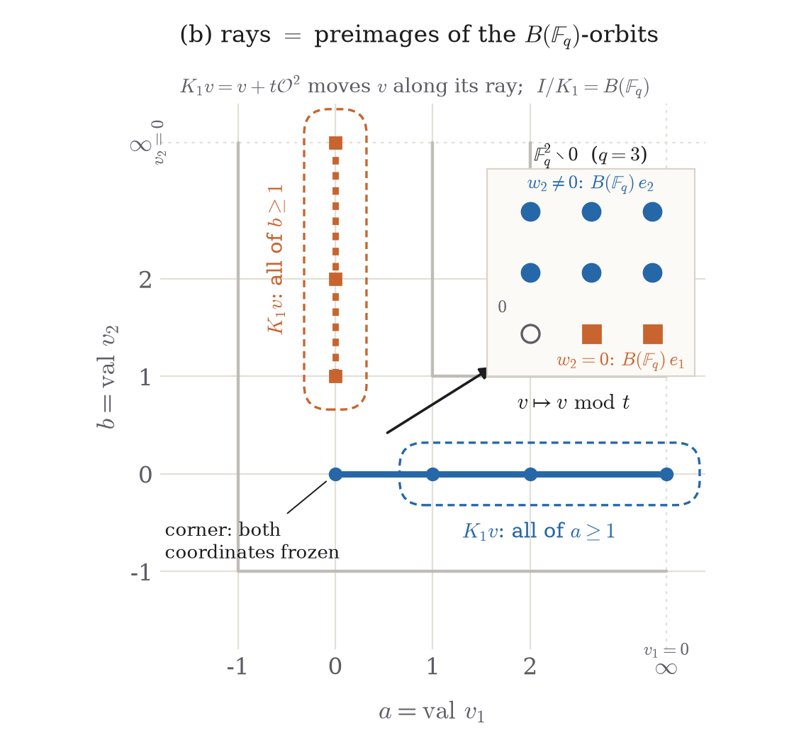
(b) Reduction to \(B(\mathbb F_q)\). By P3, the fibres of \(r_m\) are the \(K_1\)-orbits. Since \(I/K_1=B(\mathbb F_q)\), P4 identifies the \(I\)-orbits as \(r_m^{-1}(Be_j)=O_{m,j}\). For \(n=2\), these are \(\{b=m\le a\}\) and \(\{a=m<b\}\).
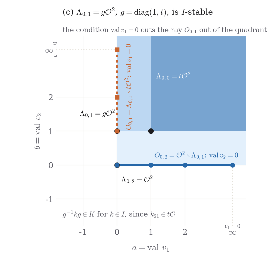
(c) Lattices and their differences. For \(k\in I\) and \(g=g_{m,j}\), \(g^{-1}kg\) has entries \(t^{-e_a}k_{ab}t^{e_b}\) with \(e_a\in\{0,1\}\) non-decreasing in \(a\); the only negative exponent occurs for \(a>j\ge b\), where \(k_{ab}\in t\mathcal O\). So \(I\subseteq gKg^{-1}\) and \(\Lambda_{m,j}=g\mathcal O^n\) is \(I\)-stable. The difference \(\Lambda_{m,j}\setminus\Lambda_{m,j-1}\) is the set of \(v\in\Lambda_{m,j}\) with \(\operatorname{val}v_j=m\), which is \(O_{m,j}\): in the plane, a quadrant minus the next quadrant of the chain is one ray. Each \(O_{m,j}\) is a union of cosets of \(t^{m+1}\mathcal O^n\), hence open and closed in \(F^n\); in the Zariski topology of a finite-dimensional truncation \(t^{-N}\mathcal O^n/t^M\mathcal O^n\) the condition \(\operatorname{val}v_j=m\) is open in the closed set \(\Lambda_{m,j}\), whose other points are limits.
2 · Hecke translates of the basic function are lattice indicators
Lemma 2 (lattice translates). Let \(g\in G(F)\) and \(L=g\mathcal O^n\). Normalize \(\operatorname{vol}I=1\) for \(\mathcal H_I\) and \(\operatorname{vol}K=1\) for \(\mathcal H_K\).
- The following are equivalent: \(L\) is \(I\)-stable; \(I\subseteq gKg^{-1}\); \(IgK=gK\).
- If they hold, \(\mathbf 1_{gK}\in\mathcal H_I\) and $$\mathbf 1_{gK}\ast\varphi_0=[K:I]\,\mathbf 1_{L},\qquad\text{so}\qquad\mathbf 1_L\in\mathcal H_I\cdot\varphi_0 .$$
- The \(I\)-stable lattices in \(F^n\) are exactly the \(\Lambda_{m,j}\), \(m\in\mathbb Z\), \(0\le j\le n\), of the chain of lattices (Definition in 1).
- Spherical level: the \(K\)-stable lattices are exactly the \(t^m\mathcal O^n\), and \(\mathbf 1_{t^mK}\ast_K\varphi_0=\mathbf 1_{t^m\mathcal O^n}\in\mathcal H_K\cdot\varphi_0\).
So every \(I\)-stable lattice is a Hecke translate of \(\varphi_0\), and (c) says the chain lists all of them. In the building of \(\mathrm{GL}_n\), the classes of \(\Lambda_{0,j}\), \(0\le j\le n-1\), up to homothety are the vertices of the base alcove, the alcove fixed by \(I\).
Proof
- For \(k\in G(F)\): \(kL=L\iff g^{-1}kg\,\mathcal O^n=\mathcal O^n\iff g^{-1}kg\in K\), since \(K\) is the stabilizer of \(\mathcal O^n\). So \(L\) is \(I\)-stable iff \(g^{-1}Ig\subseteq K\), i.e. \(I\subseteq gKg^{-1}\). The same condition says \(kg\in gK\) for every \(k\in I\), i.e. \(IgK=gK\).
- \(\mathbf 1_{gK}\) is left \(I\)-invariant by (a) and right \(I\)-invariant because \(I\subseteq K\), so it lies in \(\mathcal H_I\). For \(h\in gK\) we have \(h\mathcal O^n=g\mathcal O^n=L\), so \(\varphi_0(h^{-1}x)=\mathbf 1_{\mathcal O^n}(h^{-1}x)=\mathbf 1_L(x)\) does not depend on \(h\). Hence $$(\mathbf 1_{gK}\ast\varphi_0)(x)=\int_{gK}\varphi_0(h^{-1}x)\,dh=\operatorname{vol}(gK)\,\mathbf 1_L(x)=[K:I]\,\mathbf 1_L(x).$$ For \(n=2\) this is the computation 4C of the classical page, with \([K:I]=q+1\).
- Each \(\Lambda_{m,j}\) is \(I\)-stable by Lemma 1(c). Conversely let \(L\) be an \(I\)-stable lattice.
- Choose the scale. Let \(m\) be the largest integer with \(L\subseteq t^m\mathcal O^n\); it exists because \(L\) is a lattice. Then \(L\) contains some \(v\) with \(\operatorname{ord}v=m\).
- \(L\supseteq t^{m+1}\mathcal O^n\). \(K_1\subseteq I\), so \(K_1v\subseteq L\). By P3, \(K_1v=v+t^{m+1}\mathcal O^n\). Subtracting \(v\in L\) gives \(t^{m+1}\mathcal O^n\subseteq L\).
- Pass to \(\mathbb F_q^n\). Hence \(t^{m+1}\mathcal O^n\subseteq L\subseteq t^m\mathcal O^n\), and \(L\) is determined by its image \(W\subseteq t^m\mathcal O^n/t^{m+1}\mathcal O^n\cong\mathbb F_q^n\) (via \(t^mu\mapsto u\bmod t\)). \(W\) is a subspace, \(W\ne0\) by (i), and \(I\) acts on the quotient through \(k\mapsto k\bmod t\), which maps onto \(B(\mathbb F_q)\). So \(W\) is a nonzero \(B(\mathbb F_q)\)-stable subspace.
- \(W\) is a coordinate subspace. Let \(j\) be the largest last nonzero coordinate of a vector of \(W\), so \(W\subseteq\langle e_1,\dots,e_j\rangle\). Pick \(w\in W\) with last nonzero coordinate \(j\). By P4, \(W\supseteq B(\mathbb F_q)w=B(\mathbb F_q)e_j\), which contains \(e_j\) and every \(e_j+e_i\), \(i\lt j\). These span \(\langle e_1,\dots,e_j\rangle\), so \(W=\langle e_1,\dots,e_j\rangle\).
- Conclude. \(\Lambda_{m,j}\) also lies between \(t^{m+1}\mathcal O^n\) and \(t^m\mathcal O^n\) and has image \(\langle e_1,\dots,e_j\rangle\) (its first \(j\) coordinates may have valuation \(m\), the others not). Two lattices between \(t^{m+1}\mathcal O^n\) and \(t^m\mathcal O^n\) with the same image are equal, so \(L=\Lambda_{m,j}\).
- Run (c) with \(K\) in place of \(I\): now \(W\) is a nonzero \(\mathrm{GL}_n(\mathbb F_q)\)-stable subspace, hence all of \(\mathbb F_q^n\), and \(L=t^m\mathcal O^n\). The formula is (b) with \(K\) in place of \(I\): \(\operatorname{vol}(t^mK)=1\).
3 · Generation at both levels, for every \(n\)
Theorem 3. For \(X=\mathbb A^n\) under \(\mathrm{GL}_n\), every \(n\ge1\) and every non-archimedean \(F\):
$$\begin{gathered}\mathcal H_K\cdot\varphi_0=C_K,\qquad\mathcal H_I\cdot\varphi_0=C_I,\\[8pt]\text{so }\ Q_X=C_I/\mathcal H_I\cdot C_K=0\qquad\text{and}\qquad Q_{X,\varphi_0}=C_I/\mathcal H_I\cdot\varphi_0=0 .\end{gathered}$$Explicitly, \(C_I\) has the basis \(\{\mathbf 1_{O_{m,j}}\}_{m\in\mathbb Z,1\le j\le n}\cup\{\mathbf 1_{t^N\mathcal O^n}\}\) (any one \(N\)), and
$$\begin{gathered}\mathbf 1_{O_{m,j}}=\mathbf 1_{\Lambda_{m,j}}-\mathbf 1_{\Lambda_{m,j-1}}=[K:I]^{-1}\big(\mathbf 1_{g_{m,j}K}-\mathbf 1_{g_{m,j-1}K}\big)\ast\varphi_0,\\[8pt]\mathbf 1_{t^N\mathcal O^n}=[K:I]^{-1}\,\mathbf 1_{t^NK}\ast\varphi_0 .\end{gathered}$$Proof
- Let \(\varphi\in C_I\). Compact support: \(\operatorname{supp}\varphi\subseteq t^{-N}\mathcal O^n\). Local constancy at \(0\): \(\varphi\) is constant on \(t^N\mathcal O^n\) for \(N\) large. \(I\)-invariance: \(\varphi\) is constant on each \(O_{m,j}\). Between \(t^{-N}\mathcal O^n\) and \(t^N\mathcal O^n\) there are \(2N\) shells and \(2Nn\) orbits, so
- and every term is in \(\mathcal H_I\cdot\varphi_0\) by Lemma 1(c) and Lemma 2(b). The same with shells \(X_m=t^m\mathcal O^n\setminus t^{m+1}\mathcal O^n\) and \(\mathbf 1_{t^mK}\ast_K\varphi_0\) gives \(C_K\). Linear independence of the listed functions: disjoint supports apart from \(\mathbf 1_{t^N\mathcal O^n}\), which is the only one nonzero at \(0\).
- \(Q_X=0\): \(\mathcal H_I\cdot C_K\supseteq\mathcal H_I\cdot\varphi_0=C_I\). The criterion (Proposition B) is confirmed in both directions.
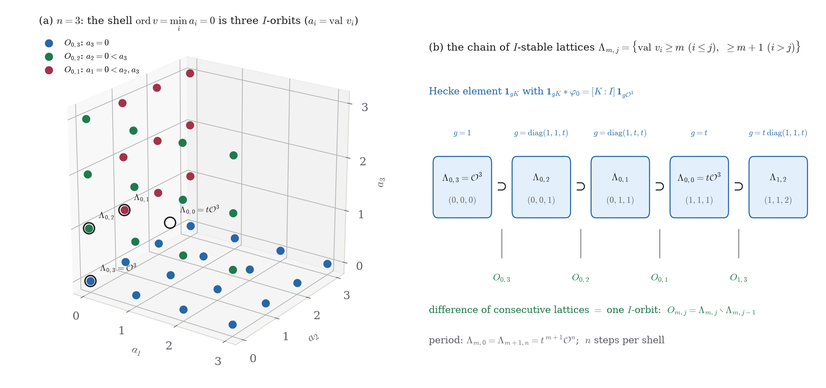
What generalizes from \(n=2\) to \(n\): the shell splits into \(n\) orbits instead of \(2\), the chain of \(I\)-stable lattices has \(n\) steps per shell instead of \(2\), and nothing else changes. Spherical generation is the special case of the chain in which only the central elements \(t^m\) are used. The pasted rank-one note proves the case \(n=2\) in row-vector conventions (its lattices \(L_m,L_m'\) are \(\Lambda_{m,2},\Lambda_{m,1}\) after exchanging the two coordinates).
4 · Why the origin matters: \(\mathbb A^2\setminus\{0\}\) against \(\mathbb A^2\)
On the punctured plane the same orbits \(O_{m,j}\) exist, but \(\mathbf 1_{\Lambda}\) is no longer compactly supported. The punctured-plane example shows that \(C_c^\infty(F^2\setminus0)^I\to\mathrm{St}^I\simeq\mathbb C\) kills \(\varphi_0\) (radial integration \(\mathcal R\) followed by \(C^\infty(\mathbb P^1)\to\mathrm{St}\)). In the valuation plane this functional is
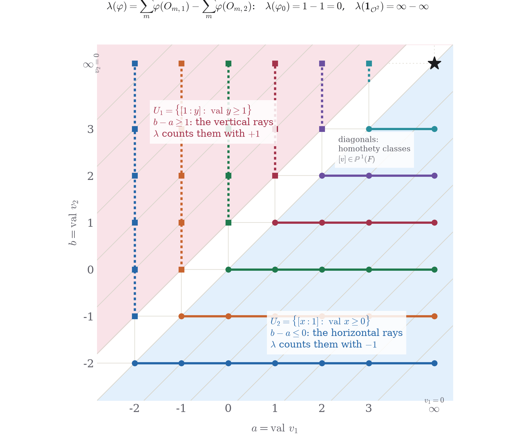
$$\begin{gathered}\lambda(\varphi)=\sum_{m\in\mathbb Z}\varphi(O_{m,1})-\sum_{m\in\mathbb Z}\varphi(O_{m,2}),\\[8pt]\lambda(\varphi_0)=1-1=0,\qquad\lambda(\mathbf 1_{\Lambda})=\infty-\infty\ \text{ (undefined)}.\end{gathered}$$Derivation
- \((\mathcal R\varphi)([v])=\int_{F^\times}\varphi(sv)\,d^\times s\) sums \(\varphi\) along the homothety class of \(v\), the diagonal \(\{(a+k,b+k)\}\) through \(\operatorname{val}v=(a,b)\). For \(b-a\ge1\) the diagonal meets only vertical rays \(O_{k,1}\), one per \(k\); for \(b-a\le0\) only horizontal rays \(O_{k,2}\). So \(\mathcal R\varphi\) is \(\sum_k\varphi(O_{k,1})\) on \(U_1=\{[1:y]:\operatorname{val}y\ge1\}\) and \(\sum_k\varphi(O_{k,2})\) on \(U_2=\{[x:1]:\operatorname{val}x\ge0\}\), the two \(I\)-orbits of \(\mathbb P^1(F)\); the map \(C^\infty(\mathbb P^1)^I=\mathbb C\mathbf 1_{U_1}\oplus\mathbb C\mathbf 1_{U_2}\to\mathrm{St}^I\) is \(f\mapsto f(U_1)-f(U_2)\).
- \(\varphi_0=\mathbf 1_{X_0}=\mathbf 1_{O_{0,1}}+\mathbf 1_{O_{0,2}}\), one ray of each kind. A lattice contains infinitely many rays of each kind.
In representation-theoretic terms: \(0\to\mathcal S(F^2\setminus0)\to\mathcal S(F^2)\xrightarrow{\mathrm{ev}_0}\mathbb C\to0\) is exact; Theorem 3 with Lemma C of the Iwahori pages gives \(\operatorname{Hom}_G(\mathcal S(F^2),\mathrm{St})=0\), while \(\operatorname{Hom}_G(\mathcal S(F^2\setminus0),\mathrm{St})\ni\mathcal R\ne0\). So the connecting map of the long exact sequence sends \(\mathcal R\) to a nonzero class in \(\operatorname{Ext}^1_G(\mathbb C,\mathrm{St})\): the obstruction on the punctured plane is an extension of the trivial representation by \(\mathrm{St}\), and the origin absorbs it. Off the origin, \(\mathbb A^n\setminus0=\mathrm{GL}_n/\mathrm{Mir}_n\) is horospherical (\(\mathrm{Mir}_n\supseteq N\)), which is where the Steinberg-type quotients come from.
5 · The two levels side by side
| spherical level \(K\) | Iwahori level \(I\) | |
|---|---|---|
| orbits on \(F^n\setminus0\) | shells \(X_m\), one per \(m\in\mathbb Z\) | \(O_{m,j}\), \(n\) per shell |
| stable lattices | \(t^m\mathcal O^n\) | the chain \(\Lambda_{m,j}\), \(n\) per shell |
| Hecke translate of \(\varphi_0\) | \(\mathbf 1_{t^mK}\ast\varphi_0=\mathbf 1_{t^m\mathcal O^n}\) | \(\mathbf 1_{g_{m,j}K}\ast\varphi_0=[K:I]\mathbf 1_{\Lambda_{m,j}}\) |
| orbit indicator | \(\mathbf 1_{t^m\mathcal O^n}-\mathbf 1_{t^{m+1}\mathcal O^n}\) | \(\mathbf 1_{\Lambda_{m,j}}-\mathbf 1_{\Lambda_{m,j-1}}\) |
| generation | holds | holds; \(Q_X=0\) |
6 · The sheaf statement (sketch)
Over \(k=\mathbb C\), \(LX=L\mathbb A^n=\varinjlim_Nt^{-N}\mathcal O^n\) with \(\mathcal O=k[[t]]\), each \(t^{-N}\mathcal O^n=\varprojlim_Mt^{-N}\mathcal O^n/t^M\mathcal O^n\) a pro-finite-dimensional affine space. The \(I\)-orbits are the \(O_{m,j}\) and \(\{0\}\) of Lemma 1, now locally closed sub-ind-schemes with connected stabilizers (the stabilizer of \(t^me_j\) in \(I\) is the preimage of the connected group \(\operatorname{Stab}_{B}(e_j)\) under \(I\to B\), a pro-unipotent extension), and
$$\overline{O_{m,j}}=\Lambda_{m,j}\supseteq O_{m,j}\sqcup\Lambda_{m,j-1}\supseteq\cdots\supseteq\{0\},$$so every orbit closure contains infinitely many orbits and the point \(0\).
Proposition 4 (sketch). \(\Delta_{g_{m,j}K}\ast_K\mathrm{IC}_0=\underline k_{\Lambda_{m,j}}\) (no shift), the standard objects \(\Delta_{m,j}:=j_!\underline k_{O_{m,j}}\) lie in \(\mathcal C_I^{\mathrm{Iwa}}\), and \(\mathcal C_I^{\mathrm{Iwa}}=\mathcal C_I\), i.e. \(\mathcal D_c(I\backslash L\mathbb A^n)^{\mathrm{Sat}}=\mathcal D_c(I\backslash L\mathbb A^n)\); likewise \(\mathcal C^{\mathrm{Sat}}=\mathcal C\) at spherical level.
Argument, and what it assumes
- Translates. For \(g=g_{m,j}\) the cell \(IgK/K\) is the single point \(gK\) (Lemma 2(a)), so the convolution space \(IgK\times^KL^+X=gK\times^K\mathcal O^n\) maps isomorphically onto \(g\mathcal O^n=\Lambda_{m,j}\) under the action map; \(m_{K*}\) of the constant sheaf is \(\underline k_{\Lambda_{m,j}}\). Same for \(t^mK\) at spherical level: \(V_{(m,\dots,m)}\ast\mathrm{IC}_0=\underline k_{t^m\mathcal O^n}\).
- Standards. \(O_{m,j}\) is open in \(\Lambda_{m,j}\) with closed complement \(\Lambda_{m,j-1}\); the triangle \(j_!j^*\to\mathrm{id}\to i_*i^*\) for \(\underline k_{\Lambda_{m,j}}\) reads \(\Delta_{m,j}\to\underline k_{\Lambda_{m,j}}\to\underline k_{\Lambda_{m,j-1}}\), and (T1) puts \(\Delta_{m,j}\) in the thick span. At spherical level the same triangle with \(X_m\subseteq t^m\mathcal O^n\) gives \(j_!\underline k_{X_m}\).
- Everything. An object of \(\mathcal C_I=\mathcal D_c(I\backslash L\mathbb A^n)\) is supported on some \(t^{-N}\mathcal O^n\) and, by the coherence condition tested on smooth charts, is pulled back from a finite level \(t^{-N}\mathcal O^n/t^M\mathcal O^n\), a finite-dimensional vector space with an action of the finite-dimensional group \(I/I_M\) (\(I_M=1+t^MM_n(\mathcal O)\)). Its \(I/I_M\)-orbits are the images of the finitely many \(O_{m,j}\) with \(-N\le m<M\), all with connected stabilizers, and the point \(0\); this is a finite stratification, and the paper's generation-by-standards argument (its Proposition on standard objects, with the orbit-filtration hypothesis (H1)(b) replaced by the finite stratification at level \(M\)) gives that the finite-level category is the thick span of its standards. Pulled back to \(LX\), these are the \(\Delta_{m,j}\) and \(\underline k_{t^M\mathcal O^n}=\Delta_{t^MK}\ast\mathrm{IC}_0\).
- Assumed, not checked here: that \(\mathcal D_c(I\backslash L\mathbb A^n)\) is the colimit over \(N,M\) of the finite-level equivariant categories with these pullbacks (the paper's Definition of coherent \(\mathcal D\)-modules on a placid ind-scheme, and its Example on placid presentations, make this the expected statement), and the standard-generation lemma at finite level. Both are routine for a vector space; neither is written in the paper for a non-homogeneous \(X\). The analogue for functions is Theorem 3, where the finite-level statement is the local constancy at \(0\).
So \(\mathbb A^n\) behaves like \(\mathbb G_m\) and unlike the group case: the Iwahori-generated part is everything. The argument above is Proposition IV.1: the conditions I1–I3 are checked one finite level \(t^{-N}\mathcal O^n/t^M\mathcal O^n\) at a time, where the pieces are the \(O_{m,j}\) with \(m<M\) and the tail \(t^M\mathcal O^n\). The paper's route to \(\mathcal C^{\mathrm{Sat}}=\mathcal C\) through (H1)–(H5) does not apply, because its orbit-filtration hypothesis (H1)(a), finitely many orbits in each closure, fails for \(\mathbb A^n\) (the closure of \(X_m\) is \(t^m\mathcal O^n\)); the chain of lattices replaces it.
7 · Does the main theorem of the paper include \(X=\mathbb A^n\)?
The paper's gives, for \(X\) in its class of satisfying its (a)–(c),
$$\begin{gathered}\mathbb L^{\mathrm{Sat}}:\ \mathcal D_c(I\backslash LX)^{\mathrm{Sat}}\xrightarrow{\ \sim\ }\operatorname{Perf}\big(\mathrm{sh}^{1/2}(\tilde{\check{\mathfrak g}}{}^*(2)\times_{\check{\mathfrak g}^*(2)}\check M)/\check G\big),\\[8pt]\mathcal D_c(I\backslash LX)^{\mathrm{Sat}}=\operatorname{Thick}\{\mathcal F\ast\mathrm{IC}_0:\ \mathcal F\in\mathcal D_c(I\backslash\operatorname{Gr})\}=\mathcal C_I^{\mathrm{Iwa}}\qquad(\text{I}'\text{(a)}).\end{gathered}$$| requirement | for \(\mathbb A^n\) | status |
|---|---|---|
| Definition: smooth affine spherical, connected \(B\)-stabilizers on the open orbit | \(B\cdot e_n\) open, \(\operatorname{Stab}_B(e_n)\) connected (1); \(M=T^*(2)\mathbb A^n=\mathbb A^n\oplus\mathbb A^{n*}\) | holds |
| (a) \(LX\) is an \(L^+G\)-placid ind-scheme presented by orbit closures | Chen–Yi (the paper's ) for every smooth affine spherical \(X\); here \(L\mathbb A^n=\varinjlim_mt^{-m}\mathcal O^n=\varinjlim_m\overline{X_{-m}}\) directly | holds |
| (b) \(LX\) admits a dimension theory | \(F^n\) is a Tate vector space; \(\dim(t^{-m}\mathcal O^n:\mathcal O^n)=mn\). The paper's cites Chen–Yi only for symmetric \(X\) | holds; one sentence to add |
| (c) the for \((\mathrm{GL}_n,\mathbb A^n)\) | not among the paper's (group, \(M_n\) under \(\mathrm{GL}_n\times\mathrm{GL}_n\), Shalika, linear, Gan–Gross–Prasad, rank-one homogeneous). \(n=1\) is Tate's thesis, \((\mathbb G_m,\mathbb A^1)\) self-dual. For \(n\ge2\) the unramified quotients of \(\mathcal S(F^n)\) are the degenerate principal series \(\operatorname{Ind}_{P_{1,n-1}}(\chi\otimes\mathbf 1_{\mathrm{GL}_{n-1}})\), parameter \(\chi\oplus\mathrm{Sym}^{n-2}\): \(\check G_X=\mathrm{GL}_1\) with the Arthur \(\mathrm{SL}_2\) principal in \(\mathrm{GL}_{n-1}\), so \(\check M\) should be the Whittaker induction of \(T^*\mathbb A^1\) along \(P_{1,n-1}\) | open here: needs a reference or a proof |
| Section “Satake equals full”: (H1)(a) finitely many orbits in each closure | fails: \(\overline{X_m}=t^m\mathcal O^n\supseteq\bigsqcup_{m'\ge m}X_{m'}\sqcup\{0\}\) | not applicable; replaced by 6 |
Answer. \(X=\mathbb A^n\) is in the class the main theorem is stated for, and (a), (b) hold; the theorem applies to \(\mathbb A^n\) exactly when the unramified relative Langlands equivalence (c) is available for \((\mathrm{GL}_n,T^*\mathbb A^n)\), which the paper does not claim for this \(X\). When it is, the theorem describes \(\mathcal D_c(I\backslash L\mathbb A^n)^{\mathrm{Sat}}\), and by 6 (sketch; by Theorem 3 for functions) that is the whole Iwahori category, unlike the group case. The paper's own is for symmetric varieties and do not cover \(\mathbb A^n\); the lattice-chain argument is the substitute. For \(n=1\) the Iwahori statement is empty (\(I=K\), \(\tilde{\check{\mathfrak g}}{}^*=\check{\mathfrak g}^*\)).