- II · Statement
- IIa · Traces of Satake objects
- IIb · IC basis and the matrix
- IIc · Functions ⇒ sheaves
- Trace dictionary
Proposition IIb and proof
Part (b) of Proposition II: trace functions of intersection complexes are a basis, a Satake trace has the coordinates \(m_{\nu\lambda}\), and spherical generation is the spanning of the columns.
Proposition II as a paper · statement and complete proof (PDF) →
Definitions
Group data over a finite field
\(p\) is an odd prime and \(q\) a power of \(p\). \(G\) is a connected reductive group over \(\mathbb F_q\) and \(\theta\) an involution of \(G\) over \(\mathbb F_q\):
$$X=G/G^\theta,\qquad x_0=eG^\theta .$$\(S\) is a maximal \(\theta\)-split torus and \(T\supseteq S\) a \(\theta\)-stable maximal torus. Labels and the leading-term map are those of the pages:
$$\Lambda_T^+\subseteq X_*(T),\qquad\Lambda_S^+=X_*(S)\cap\Lambda_T^+,\qquad\varphi(\lambda)=\lambda-\theta(\lambda),$$with the dominance order on \(\Lambda_S^+\), in which lower sets \(\{\nu\le\mu\}\) are finite.
Sheaves over \(k=\overline{\mathbb F}_q\)
\(LX\) and \(L^+G\) are the loop space and the arc group over \(k\); the orbits are \(\mathcal O_\mu=L^+G\cdot x_\mu\) with \(\tau(x_\mu)=t^\mu\). The category is Chen–Yi's \(\ell\)-adic one:
$$\mathcal C_{K,k}=\{\text{bounded }L^+G\text{-equivariant constructible }\overline{\mathbb Q}_\ell\text{-complexes on }LX\text{, supported on finitely many orbit closures}\}.$$\(\mathrm{IC}_\nu\) is the intersection complex of \(\overline{\mathcal O_\nu}\) with constant coefficients, \(V_\lambda\) the Satake sheaf of \(\operatorname{Gr}_{\le\lambda}\), and \(\mathrm{IC}_0\) the constant sheaf on \(L^+X\):
$$\mathrm{IC}_\nu|_{\mathcal O_\nu}\simeq\overline{\mathbb Q}_\ell[\delta(\nu)],\qquad\mathcal C^{\mathrm{Sat}}_{K,k}=\operatorname{Thick}_{\mathcal C_{K,k}}\{V_\lambda\ast\mathrm{IC}_0:\lambda\in\Lambda_T^+\}.$$The Betti category \(\mathcal C_K\) of the pages is the same construction over \(\mathbb C\) with complex coefficients.
Functions over \(F=\mathbb F_q(\!(t)\!)\)
\(F=\mathbb F_q(\!(t)\!)\) has ring of integers \(\mathcal O=\mathbb F_q[\![t]\!]\). Its points are the \(\mathbb F_q\)-points of the loop spaces:
$$LX(\mathbb F_q)=X(F),\qquad LG(\mathbb F_q)=G(F),\qquad L^+G(\mathbb F_q)=K=G(\mathcal O).$$The spherical Hecke algebra \(\mathcal H_K\) consists of the compactly supported \(K\)-bi-invariant functions on \(G(F)\); it has the basis \(T_\lambda\), \(\lambda\in\Lambda_T^+\) (Cartan decomposition), and acts by convolution on the \(K\)-invariant functions on \(X(F)\), with Haar measure normalized by \(\operatorname{vol}K=1\):
$$\mathcal H_K=C_c(K\backslash G(F)/K),\qquad T_\lambda=\mathbf 1_{Kt^\lambda K},\qquad(f\ast\varphi)(x)=\sum_{gK\in G(F)/K}f(g)\,\varphi(g^{-1}x),$$ $$C_K=C_c^\infty(X(F))^K,\qquad\varphi_0=\mathbf 1_{X(\mathcal O)}.$$Spherical generation.
$$\text{(SG)}\qquad\mathcal H_K\ast\varphi_0=C_K.$$For a field \(E\) of characteristic \(0\), \(\mathcal H_K\ast\varphi_0\otimes E\) is the \(E\)-span of the \(\mathbb Z\)-valued functions \(T_\lambda\ast\varphi_0\) and \(C_K\otimes E\) the \(K\)-invariant compactly supported \(E\)-valued functions; (SG) does not depend on \(E\) (IIb, step 7).
Other residue fields. Proposition II needs only \(F\). Since \(\overline{\mathbb F}_{q^n}=\overline{\mathbb F}_q\), replacing \(q\) by \(q^n\) leaves \(\mathcal C_{K,k}\) and its objects unchanged and gives the same statements over \(F_n=\mathbb F_{q^n}(\!(t)\!)\), with \(K_n=G(\mathbb F_{q^n}[\![t]\!])\), \(\mathcal H_{K_n}\), \(C_{K_n}\), \((\mathrm{SG})_n\), the trace \(\operatorname{tr}_n\) of the \(n\)-th iterate of \(\Phi\) and the matrix \(m^{(n)}\) (trace dictionary). Several \(n\) at once are used only for the converse (II, limits; Proposition IX).
Weil objects and trace functions
A Weil object is a pair \((M,\Phi)\) with \(M\in\mathcal C_{K,k}\) and \(\Phi:\mathrm{Fr}^*M\xrightarrow{\sim}M\), where \(\mathrm{Fr}\) is the \(\mathbb F_q\)-linear Frobenius endomorphism of \(LX\) (coordinates raised to the \(q\)-th power), so that \(LX(\mathbb F_q)=X(F)\) is its set of fixed points. For \(x\in X(F)\) and a geometric point \(\bar x\) over it, \(\mathrm{Fr}(\bar x)=\bar x\), so \(\Phi_{\bar x}\) acts on each stalk cohomology \(\mathcal H^i(M)_{\bar x}\), and the trace function of \(M\) is
$$\operatorname{tr}(M)(x)=\sum_i(-1)^i\operatorname{tr}\big(\Phi_{\bar x},\ \mathcal H^i(M)_{\bar x}\big)\in\overline{\mathbb Q}_\ell .$$The function \(\operatorname{tr}(M)\) is \(K\)-invariant and lies in \(C_K\otimes\overline{\mathbb Q}_\ell\) (IIb, steps 1–2); it is additive on Frobenius-compatible distinguished triangles, and \(\operatorname{tr}(M[1])=-\operatorname{tr}(M)\). \(V_\lambda\), \(\mathrm{IC}_0\) and \(\mathrm{IC}_\nu\) carry canonical Weil structures (eigenvalue \(1\) on the lowest stalk cohomology of the open stratum, no Tate twist), and \(V_\lambda\ast\mathrm{IC}_0\) the induced one. The trace dictionary: properties, conventions and sources →
Multiplicity spaces and the matrix \(m\)
By D2 each Satake object is a finite sum of shifted intersection complexes. With \(P_i={}^p\mathcal H^i(V_\lambda\ast\mathrm{IC}_0)\), the \(i\)-th perverse cohomology sheaf, the multiplicity space \(E_{\nu,i}(\lambda)\) counts the copies of \(\mathrm{IC}_\nu[-i]\):
$$V_\lambda\ast\mathrm{IC}_0\simeq\bigoplus_{\nu,i}\mathrm{IC}_\nu[-i]\otimes E_{\nu,i}(\lambda),\qquad E_{\nu,i}(\lambda)=\operatorname{Hom}\big(\mathrm{IC}_\nu,P_i\big).$$The Weil structure induces the Frobenius \(A_{\nu,i}(\lambda)\in\mathrm{GL}(E_{\nu,i}(\lambda))\) (IIb, step 4). The matrix has rows indexed by orbit labels and columns by Hecke labels:
$$m_{\nu\lambda}=\sum_i(-1)^i\operatorname{tr}A_{\nu,i}(\lambda)\qquad(\nu\in\Lambda_S^+,\ \lambda\in\Lambda_T^+).$$Each column \((m_{\nu\lambda})_\nu\) has finitely many nonzero entries. "Every row is nonzero" and "the columns span \(\bigoplus_{\Lambda_S^+}\overline{\mathbb Q}_\ell\)" are the two conditions compared on these pages.
Proposition I (summand criterion)
Assume H1–H3 and that every \(V_\lambda\ast\mathrm{IC}_0\) is a finite sum of shifted \(\mathrm{IC}_\nu\) with constant coefficients. Put
$$\mathcal M=\{\mu\in\Lambda_S^+:\mathrm{IC}_\mu[s]\text{ is a direct summand of some }V_\lambda\ast\mathrm{IC}_0,\ s\in\mathbb Z\}.$$Then
$$\mathcal C_K^{\mathrm{Sat}}=\operatorname{Thick}\{\mathrm{IC}_\nu:\nu\in\mathcal M\},\qquad\mathcal C_K^{\mathrm{Sat}}=\mathcal C_K\iff\mathcal M=\Lambda_S^+ .$$So \(\mathcal M\) is the set of labels whose intersection complex occurs, up to shift, as a direct summand of a Satake object, and the sheaf statement \(\mathcal C_K^{\mathrm{Sat}}=\mathcal C_K\) is the statement \(\mathcal M=\Lambda_S^+\). For \(\mathcal C_{K,k}\): H1 follows from D0, H2 from D1, H3 from the connectedness hypothesis. Proposition I · proof →
Hypotheses (R), (C) and inputs D0–D3, D5
(R) · Rationality.
\(G\), \(\theta\) and \(X\) are defined over \(\mathbb F_q\), \(q\) odd; \(T\supseteq S\) is split over \(\mathbb F_q\); and \(G\) has a \(\theta\)-stable Borel pair \((B_0,T_0)\) over \(\mathbb F_q\) with \(T_0\) split (Chen–Yi, §8.2). Then every \(t^\mu\), \(\mu\in\Lambda_S\), lies in \(S(F)\).(C) · Connectedness.
$$G^\theta\ \text{ and }\ Z_{G^\theta}(S)\ \text{ are connected}.$$D0 · Orbit geometry over \(k\).
For \(p\ne2\) (Chen–Yi, Prop. 17, Thm 18 and the pages' Proposition III): $$LX(k)=\bigsqcup_{\mu\in\Lambda_S^+}\mathcal O_\mu(k),\quad\tau(x_\mu)=t^\mu,\qquad\overline{\mathcal O_\mu}=\bigsqcup_{\nu\le\mu}\mathcal O_\nu,\qquad\operatorname{supp}(V_\lambda\ast\mathrm{IC}_0)\subseteq\overline{\mathcal O_{\varphi(\lambda)}},$$ $$\operatorname{Stab}_{L^+G}(x_\mu)=Z_{G^\theta}(\mu)\ltimes U_\mu,\ \ U_\mu\ \text{pro-unipotent},\qquad\pi_0Z_{G^\theta}(\mu)=1\ \text{ for all }\mu\ \text{ under (C)}.$$D1 · Traces and t-structure.
Proper base change and the Grothendieck–Lefschetz trace formula on the fibres of the convolution map; Chen–Yi's sheaf theory on \(L^+G\backslash LX\) (App. A.5) with a Frobenius-compatible perverse t-structure of finite length whose simple objects are the \(\mathrm{IC}_\nu\), \(\operatorname{End}(\mathrm{IC}_\nu)=\overline{\mathbb Q}_\ell\).D2 · Decomposition.
\(V_\lambda\ast\mathrm{IC}_0\) is pure, and over \(k\) $$V_\lambda\ast\mathrm{IC}_0\simeq\bigoplus_{\nu,i}\mathrm{IC}_\nu[-i]\otimes E_{\nu,i}(\lambda),\qquad\dim E_{\nu,i}(\lambda)\lt\infty$$ (Sun, Thm 1.2, on finite-type equivariant models; Chen–Yi, Prop. 70 and the proof of Thm 93).D3 · Lang's theorem.
For \(L^+G=\varprojlim_mG(\mathbb F_q[t]/t^m)\) and its stabilizers: $$H^1(\mathbb F_q,L^+G)=1,\qquad H^1\big(\mathbb F_q,\operatorname{Stab}_{L^+G}(x_\mu)\big)=H^1\big(\mathbb F_q,\pi_0\operatorname{Stab}_{L^+G}(x_\mu)\big).$$D5 · Comparison with \(\mathbb C\).
The statement "\(\mathrm{IC}_\mu\) is a summand of \(V_\lambda\ast\mathrm{IC}_0\)", which lives on the finite-type model \(\operatorname{Gr}_{\le\lambda}\mathbin{\widetilde\times}\overline{\mathcal O_0}\to\overline{\mathcal O_{\varphi(\lambda)}}\), has the same answer over \(\overline{\mathbb F}_q\) and over \(\mathbb C\) (BBD §6.1; Bezrukavnikov–Finkelberg, Prop. 5, for \(p\) outside a finite set). Used only for the Betti form of the conclusion.
Proposition IIb · the IC basis and the matrix \(m\)
Setting. \(X=G/G^\theta\) over \(\mathbb F_q\), \(q\) odd, with (R) and (C); sheaves in \(\mathcal C_{K,k}\) over \(k=\overline{\mathbb F}_q\), with Satake objects \(V_\lambda\ast\mathrm{IC}_0\) and intersection complexes \(\mathrm{IC}_\nu\). The functions live on \(X(F)\), \(F=\mathbb F_q(\!(t)\!)\):1
- \(K=G(\mathbb F_q[\![t]\!])\), the stabilizer of the base point of \(\operatorname{Gr}\); \(LX(\mathbb F_q)=X(F)\).
- \(\mathcal H_K=C_c(K\backslash G(F)/K)\), the spherical Hecke algebra, with basis \(T_\lambda=\mathbf 1_{Kt^\lambda K}\), \(\lambda\in\Lambda_T^+\), acting by convolution.
- \(C_K=C_c^\infty(X(F))^K\), the basic function \(\varphi_0=\mathbf 1_{X(\mathbb F_q[\![t]\!])}\), and (SG): \(\mathcal H_K\ast\varphi_0=C_K\).
- \(\operatorname{tr}\), the alternating trace of Frobenius on stalks: a Weil object \(M\) of \(\mathcal C_{K,k}\) gives \(\operatorname{tr}(M):X(F)\to\overline{\mathbb Q}_\ell\).
1 Only \(F=\mathbb F_q(\!(t)\!)\) is needed, for an arbitrary odd \(q\). Replacing \(q\) by \(q^n\) gives the same statements over \(\mathbb F_{q^n}(\!(t)\!)\) with the same sheaves (Definitions, other residue fields).
Write \(V_\lambda\ast\mathrm{IC}_0\simeq\bigoplus_{\nu,i}\mathrm{IC}_\nu[-i]\otimes E_{\nu,i}(\lambda)\) (D2), and let \(A_{\nu,i}(\lambda)\) be the Frobenius of the multiplicity space \(E_{\nu,i}(\lambda)\) (step 4).
Claim. Assume D0–D3.
- Basis. \(\{\operatorname{tr}\mathrm{IC}_\nu\}_{\nu\in\Lambda_S^+}\) is a basis of \(C_K\otimes\overline{\mathbb Q}_\ell\), unitriangular in the orbit basis: $$\operatorname{tr}\mathrm{IC}_\nu=(-1)^{\delta(\nu)}\mathbf 1_{\mathcal O_\nu(\mathbb F_q)}+\sum_{\nu'\lt\nu}c_{\nu'\nu}\mathbf 1_{\mathcal O_{\nu'}(\mathbb F_q)}.$$
- Expansion. For every \(\lambda\in\Lambda_T^+\), $$\operatorname{tr}(V_\lambda\ast\mathrm{IC}_0)=\sum_\nu m_{\nu\lambda}\operatorname{tr}\mathrm{IC}_\nu,\qquad m_{\nu\lambda}=\sum_i(-1)^i\operatorname{tr}A_{\nu,i}(\lambda),$$ so \(m_{\nu\lambda}=0\) when \(\mathrm{IC}_\nu\) is not a shifted summand of \(V_\lambda\ast\mathrm{IC}_0\).
- Columns. (SG) holds if and only if the columns \((m_{\nu\lambda})_{\nu\in\Lambda_S^+}\), \(\lambda\in\Lambda_T^+\), span \(\bigoplus_{\Lambda_S^+}\overline{\mathbb Q}_\ell\).
(i) is proved in steps 1–3, (ii) in steps 4–5, (iii) in steps 6–7, which also use part (a) from IIa. Used by IIc.
Sources
References
- Chen–Yi, Orbit closures in loop spaces of symmetric varieties, v4: Proposition 17 and Theorem 18 (D0), §8.2 and §8.2.3 (Weil structures, the unitriangular basis), Proposition 70 and the proof of Theorem 93 (D2), Theorem 87 (constant coefficients), App. A.5 (D1), §1.2.6 (characteristic).
- Zhu, An introduction to affine Grassmannians and the geometric Satake equivalence, v2: §5.6, Lemma 5.6.1 and (5.6.2) (step 2); §A.1.4 (finite-type quotients, step 1).
- Laumon, Transformation de Fourier, constantes d'équations fonctionnelles et conjecture de Weil, Publ. Math. IHÉS 65 (1987): §1.1, the fonctions–faisceaux dictionary (1.1.1)–(1.1.1.4) and Theorem 1.1.2.
- Milne, Algebraic Groups, version 2.00 (2015): Proposition 27.54 and Corollaries 27.55–27.56, Lang's theorem (D3).
- A. Beilinson, J. Bernstein and P. Deligne, Faisceaux pervers, Astérisque 100 (1982): Theorem 4.3.1, Theorem 5.4.5 and Corollary 5.4.6, §6.1. Sun, v3, Theorem 1.2, for stacks.
- Sakellaridis, Spherical functions on spherical varieties, v3: §1.1, Theorem 8.0.2, Example 8.0.1, Corollary 8.0.4. Bezrukavnikov–Finkelberg, v2, §6.5, Proposition 5 (D5).
- Run nodes: A4-6, A3-10, A1-6 (three write-ups of one proof), A7-14 (their audit), A4-7 (converse), A4-12 (fields and levels), A1-8 and A7-16 (three fields, two bridges; its remark on the SO₂-model is corrected by C-5 and not used here).
References checked 17 October 2026. The reader in D holds located extracts.
Proof
Steps 1–2 give the orbit basis of \(C_K\), step 3 the IC basis (i), steps 4–5 the coefficients (ii). Step 6 is a lemma of linear algebra, and step 7 proves (iii) with it, one direction at a time.
-
Rational points of each orbit form one \(K\)-orbit, so the \(K\)-orbits on \(X(F)\) are indexed by \(\Lambda_S^+\):
$$X(F)=\bigsqcup_{\mu\in\Lambda_S^+}\mathcal O_\mu(\mathbb F_q),\qquad\mathcal O_\mu(\mathbb F_q)=K\cdot x_\mu .$$Proof
- Rational representatives. By D0, \(X(F)=LX(\mathbb F_q)\subseteq\bigsqcup_\mu\mathcal O_\mu(k)\). By (R), \(t^\mu\in S(F)\); \(\tau\) is injective on points, so \(x_\mu\) is rational and each \(\mathcal O_\mu\) is Frobenius-stable.
- Cocycle. For \(y=gx_\mu\in\mathcal O_\mu(\mathbb F_q)\), \(g\in L^+G(k)\), the class of \(g^{-1}\mathrm{Fr}(g)\) in \(H^1(\mathbb F_q,\operatorname{Stab}(x_\mu))\) depends only on \(y\), and it classifies the \(K\)-orbit of \(y\) because \(H^1(\mathbb F_q,L^+G)=1\) (D3).
- Vanishing. By D0 and D3, \(H^1(\mathbb F_q,\operatorname{Stab}(x_\mu))=H^1(\mathbb F_q,\pi_0Z_{G^\theta}(\mu))=1\) under (C). So \(\mathcal O_\mu(\mathbb F_q)=K\cdot x_\mu\).
- Without (C). For \(\mathrm{SL}_2/\mathrm{SO}_2\), \(\pi_0\operatorname{Stab}(x_\mu)=\{\pm I\}\) and \(\mathcal O_\mu(\mathbb F_q)\) is two \(K\)-orbits for \(\mu\ne0\); the IC traces of step 3 then fail to span (Proposition III).
-
Each \(K\cdot x_\mu\) is compact open, so:
$$C_K=\bigoplus_{\mu\in\Lambda_S^+}\mathbb C\,\mathbf 1_{\mathcal O_\mu(\mathbb F_q)},\qquad C_K\otimes\overline{\mathbb Q}_\ell=\bigoplus_{\mu\in\Lambda_S^+}\overline{\mathbb Q}_\ell\,\mathbf 1_{\mathcal O_\mu(\mathbb F_q)} .$$Proof
- Compact. \(K\) is compact, so \(K\cdot x_\mu\) is.
- Open. The orbit map \(G\to X\), \(g\mapsto gx_\mu\), is smooth (its fibres are torsors under the smooth stabilizer, \(p\ne2\)), so it is open on \(F\)-points; \(K\) is open in \(G(F)\).
- Basis. A \(K\)-invariant function is constant on each orbit; compact support meets finitely many open orbits. So the indicators span, and they are independent because the orbits are disjoint.
-
\(\operatorname{tr}\mathrm{IC}_\nu\) is not an indicator. It is \(K\)-invariant, so constant on each orbit: \((-1)^{\delta(\nu)}\) on its own orbit, the stalk trace \(c_{\nu'\nu}\) at \(x_{\nu'}\) on each smaller orbit of its closure, and \(0\) elsewhere:
$$\operatorname{tr}\mathrm{IC}_\nu=(-1)^{\delta(\nu)}\mathbf 1_{\mathcal O_\nu(\mathbb F_q)}+\sum_{\nu'\lt\nu}c_{\nu'\nu}\mathbf 1_{\mathcal O_{\nu'}(\mathbb F_q)},\qquad c_{\nu'\nu}=\operatorname{tr}\mathrm{IC}_\nu(x_{\nu'})=\sum_j(-1)^j\operatorname{tr}\big(\Phi_{x_{\nu'}},\mathcal H^j(\mathrm{IC}_\nu)_{x_{\nu'}}\big).$$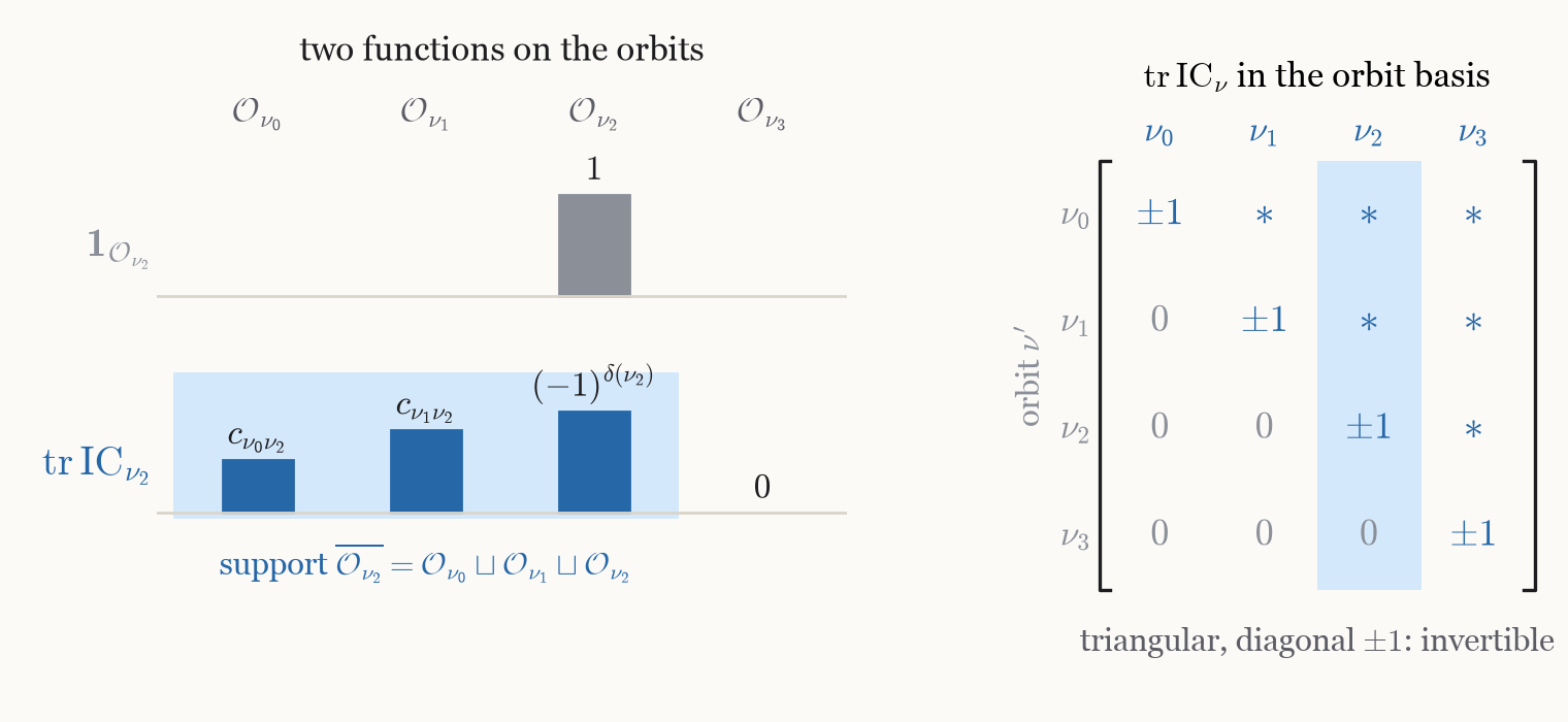
Figure 1. \(\operatorname{tr}\mathrm{IC}_{\nu_2}\) is \(\pm1\) on its own orbit and generally nonzero below it, so the IC traces form a second, triangular basis (schematic: orbits drawn as a chain, heights illustrative). Proof
- Support. \(\operatorname{supp}\mathrm{IC}_\nu=\overline{\mathcal O_\nu}=\bigsqcup_{\nu'\le\nu}\mathcal O_{\nu'}\) (D0), a finite union. The Weil structure is \(L^+G\)-equivariant, so \(\operatorname{tr}\mathrm{IC}_\nu\) is \(K\)-invariant; by step 1 it is constant on \(\mathcal O_{\nu'}(\mathbb F_q)=K\cdot x_{\nu'}\), with value \(c_{\nu'\nu}\).
- Leading term. On \(\mathcal O_\nu\), \(\mathrm{IC}_\nu=\overline{\mathbb Q}_\ell[\delta(\nu)]\) with Frobenius \(1\) (canonical Weil structure), so its trace is \((-1)^{\delta(\nu)}\).
- Basis. On a finite lower set \(L\), the IC traces \(\{\operatorname{tr}\mathrm{IC}_\nu\}_{\nu\in L}\) and the indicators \(\{\mathbf 1_{\mathcal O_\nu}\}_{\nu\in L}\) are related by a triangular matrix with diagonal \(\pm1\), so they span the same space. Every finite set of labels lies in a finite lower set, so the IC traces span \(C_K\otimes\overline{\mathbb Q}_\ell\) and are independent. Chen–Yi, §8.2.3, prove the same triangularity in the Grothendieck group.
- Why this basis. Any basis would turn \((\mathrm{SG})\) into a statement about columns (step 6). In the IC basis the coordinates of a Satake trace are the multiplicity traces \(m_{\nu\lambda}\) (step 5), and a nonzero one gives a summand (IIc).
-
Fix \(\lambda\). Three objects are attached to the Satake object \(V_\lambda\ast\mathrm{IC}_0\); Figure 2 shows them for one example.
Table 2. Object and What it is and In Figure 2 Object What it is In Figure 2 \(P_i={}^p\mathcal H^i(V_\lambda\ast\mathrm{IC}_0)\) the \(i\)-th perverse cohomology sheaf; \(V_\lambda\ast\mathrm{IC}_0\simeq\bigoplus_iP_i[-i]\) (D2) column \(i\) \(E_{\nu,i}(\lambda)=\operatorname{Hom}(\mathrm{IC}_\nu,P_i)\) multiplicity space: \(P_i\simeq\bigoplus_\nu\mathrm{IC}_\nu\otimes E_{\nu,i}(\lambda)\), and \(\dim E_{\nu,i}(\lambda)\) is the number of copies of \(\mathrm{IC}_\nu[-i]\) boxes in cell \((\nu,i)\) \(A_{\nu,i}(\lambda)\) Frobenius of \(E_{\nu,i}(\lambda)\), defined below the letters \(\alpha,\beta,\gamma\) \(P_i\) inherits a Weil structure \(\Phi_i:\mathrm{Fr}^*P_i\to P_i\), and \(\mathrm{IC}_\nu\) has its canonical one, \(\Phi_\nu\). A map \(f:\mathrm{IC}_\nu\to P_i\) is moved by Frobenius to another such map:
$$A_{\nu,i}(\lambda)f=\Phi_i\circ\mathrm{Fr}^*(f)\circ\Phi_\nu^{-1}:\quad\mathrm{IC}_\nu\xrightarrow{\ \Phi_\nu^{-1}\ }\mathrm{Fr}^*\mathrm{IC}_\nu\xrightarrow{\ \mathrm{Fr}^*f\ }\mathrm{Fr}^*P_i\xrightarrow{\ \Phi_i\ }P_i .$$So the Frobenius of \(P_i\) is the canonical one on each \(\mathrm{IC}_\nu\), twisted by \(A_{\nu,i}(\lambda)\) on its multiplicity space, and traces multiply:
$$\Phi_i=\bigoplus_\nu\Phi_\nu\otimes A_{\nu,i}(\lambda),\qquad\operatorname{tr}P_i=\sum_\nu\operatorname{tr}A_{\nu,i}(\lambda)\cdot\operatorname{tr}\mathrm{IC}_\nu .$$Example. If \(E_{\nu,i}(\lambda)\) is a line, \(A_{\nu,i}(\lambda)\) is a scalar \(\alpha\): that copy of \(\mathrm{IC}_\nu\) is \(\mathrm{IC}_\nu\) with its Frobenius multiplied by \(\alpha\) (a Tate twist \(\mathrm{IC}_\nu(-j)\) has \(\alpha=q^j\)), and its trace is \(\alpha\operatorname{tr}\mathrm{IC}_\nu\).
Proof
- Constant coefficients. D2 gives \(V_\lambda\ast\mathrm{IC}_0\simeq\bigoplus_{\nu,i}\mathrm{IC}_\nu[-i]\otimes E_{\nu,i}(\lambda)\) with constant coefficients: an equivariant local system on \(\mathcal O_\nu\) is a representation of \(\pi_0\operatorname{Stab}(x_\nu)=1\) (D0).
- Weil structure on \(P_i\). The perverse t-structure is Frobenius-stable (D1), so \(\Phi\) induces \(\Phi_i\) on \(P_i\).
- Evaluation. \(\mathrm{ev}:\bigoplus_\nu\mathrm{IC}_\nu\otimes E_{\nu,i}(\lambda)\to P_i\), \(x\otimes f\mapsto f(x)\), is an isomorphism: \(P_i\) is semisimple (D2), \(\operatorname{End}(\mathrm{IC}_\nu)=\overline{\mathbb Q}_\ell\) and \(\operatorname{Hom}(\mathrm{IC}_\nu,\mathrm{IC}_{\nu'})=0\) for \(\nu\ne\nu'\) (D1).
- Frobenius. On the summand \(\mathrm{Fr}^*\mathrm{IC}_\nu\otimes f\): \(\mathrm{ev}\circ(\Phi_\nu\otimes A_{\nu,i}(\lambda))\) is \((A_{\nu,i}(\lambda)f)\circ\Phi_\nu=\Phi_i\circ\mathrm{Fr}^*(f)\), which is \(\Phi_i\circ\mathrm{Fr}^*(\mathrm{ev})\). On stalks the trace of \(\Phi_\nu\otimes A\) on \(\mathcal H^j(\mathrm{IC}_\nu)_{\bar x}\otimes E\) is \(\operatorname{tr}\Phi_\nu\cdot\operatorname{tr}A\).
-
\(\operatorname{tr}\) is additive and turns the shift \([-i]\) into the sign \((-1)^i\); with step 4, collecting the terms of each \(\mathrm{IC}_\nu\) gives the column of \(\lambda\):
$$\operatorname{tr}(V_\lambda\ast\mathrm{IC}_0)=\sum_i(-1)^i\operatorname{tr}P_i=\sum_\nu\underbrace{\Big(\sum_i(-1)^i\operatorname{tr}A_{\nu,i}(\lambda)\Big)}_{m_{\nu\lambda}}\operatorname{tr}\mathrm{IC}_\nu .$$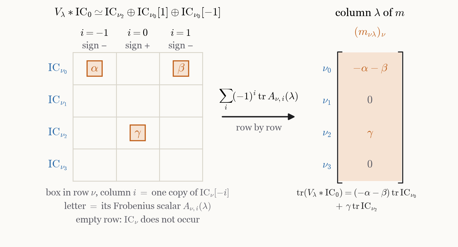
Figure 2. A box in row \(\nu\), column \(i\) is one copy of \(\mathrm{IC}_\nu[-i]\) in \(V_\lambda\ast\mathrm{IC}_0\), its letter the Frobenius scalar \(A_{\nu,i}(\lambda)\); each row sums, with signs \((-1)^i\), to one entry of the column (schematic). - Row \(\nu_0\). Two copies of \(\mathrm{IC}_{\nu_0}\): \(\mathrm{IC}_{\nu_0}[1]\) in \(P_{-1}\), scalar \(\alpha\), and \(\mathrm{IC}_{\nu_0}[-1]\) in \(P_1\), scalar \(\beta\). Their traces are \((-1)^{-1}\alpha\operatorname{tr}\mathrm{IC}_{\nu_0}\) and \((-1)^1\beta\operatorname{tr}\mathrm{IC}_{\nu_0}\), so \(m_{\nu_0\lambda}=-\alpha-\beta\).
- Row \(\nu_2\). One copy, \(\mathrm{IC}_{\nu_2}\) in \(P_0\), scalar \(\gamma\): \(m_{\nu_2\lambda}=\gamma\).
- Rows \(\nu_1\), \(\nu_3\). Empty: these ICs do not occur, so \(m_{\nu_1\lambda}=m_{\nu_3\lambda}=0\).
Proof
- Additivity. \(\operatorname{tr}\) is additive along the Frobenius-compatible perverse truncation triangles of \(V_\lambda\ast\mathrm{IC}_0\), and \(\operatorname{tr}(P[-i])=(-1)^i\operatorname{tr}(P)\) (Laumon, (1.1.1.1)): the first equality.
- Each \(P_i\). \(\operatorname{tr}P_i=\sum_\nu\operatorname{tr}A_{\nu,i}(\lambda)\operatorname{tr}\mathrm{IC}_\nu\) (step 4): the second.
- Finite columns. The sum in D2 is finite, so only finitely many \(E_{\nu,i}(\lambda)\) are nonzero.
- Vanishing. If every \(E_{\nu,i}(\lambda)\) is zero, \(m_{\nu\lambda}=0\). The converse can fail: eigenvalues \(\alpha\) and \(-\alpha\) on one \(E_{\nu,i}(\lambda)\) cancel. It is never used.
-
Linear algebra over any field \(E\). Let \(U\) have a basis \((b_\nu)_{\nu\in I}\). The coordinate map is an isomorphism:
$$\kappa:U\xrightarrow{\ \sim\ }\bigoplus_{\nu\in I}E,\qquad\sum_\nu x_\nu b_\nu\longmapsto(x_\nu)_{\nu\in I},\qquad\kappa^{-1}:(x_\nu)_{\nu\in I}\longmapsto\sum_\nu x_\nu b_\nu .$$For a matrix \(m=(m_{\nu\lambda})_{\nu\in I,\lambda\in J}\) with finitely supported columns put \(w_\lambda=\sum_\nu m_{\nu\lambda}b_\nu\). Then \(\kappa(w_\lambda)=(m_{\nu\lambda})_{\nu\in I}\) is the \(\lambda\)-th column of \(m\), and
$$\kappa\big(\operatorname{span}_\lambda w_\lambda\big)=\operatorname{span}_\lambda(m_{\nu\lambda})_{\nu\in I},\qquad\operatorname{span}_\lambda w_\lambda=U\iff\operatorname{span}_\lambda(m_{\nu\lambda})_{\nu\in I}=\bigoplus_{\nu\in I}E .$$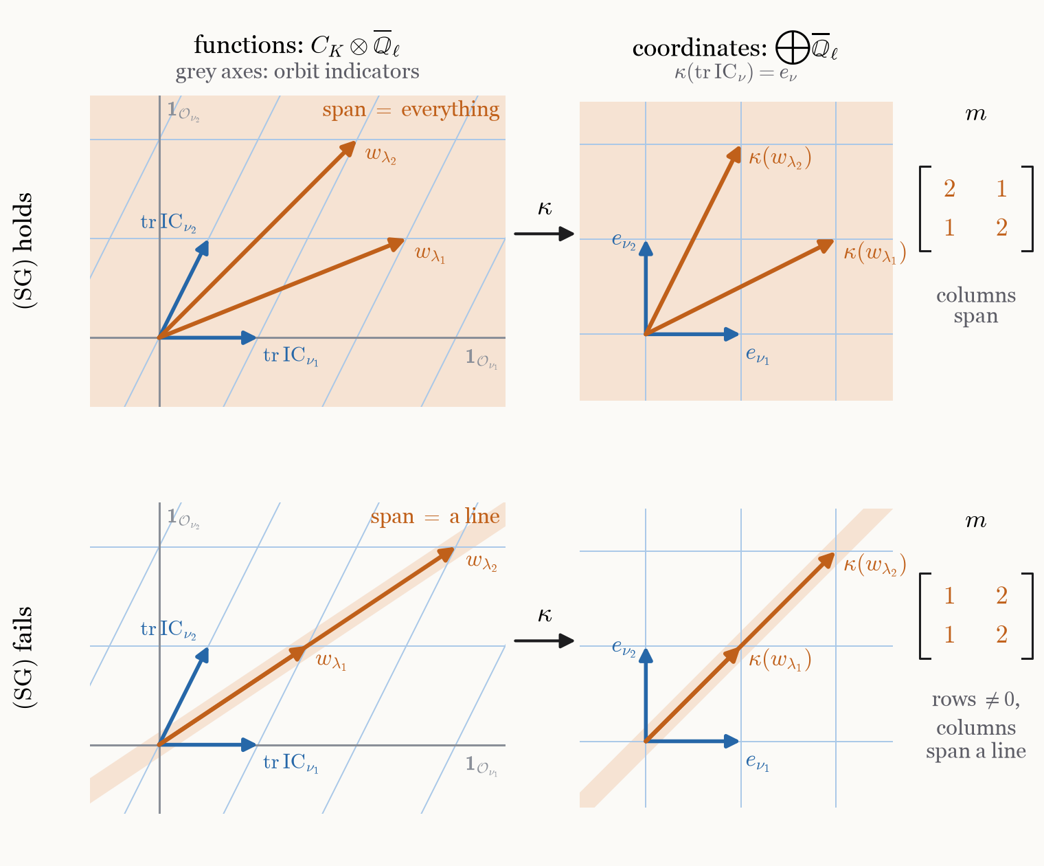
Figure 3. \(\kappa\) straightens the IC grid and sends the Satake traces \(w_\lambda\) to the columns \(\kappa(w_\lambda)\), so their span is everything exactly when the column span is (two orbits; the bottom \(m\) is hypothetical). Proof
- \(\kappa\) is well defined and linear. The \(b_\nu\) span, so every \(u\in U\) is a finite combination \(\sum_\nu x_\nu b_\nu\); they are independent, so the \(x_\nu\) are unique. Coordinates of \(au+a'u'\) are \(ax_\nu+a'x'_\nu\).
- \(\kappa\) is an isomorphism. \(\iota(x_\nu)_\nu=\sum_\nu x_\nu b_\nu\) is a finite sum, so \(\iota\) is defined on \(\bigoplus_IE\). \(\iota\kappa(u)=u\) by definition of the coordinates, and \(\kappa\iota(x)=x\) by their uniqueness. So \(\kappa^{-1}=\iota\).
- Spans. \(\kappa\big(\sum_\lambda a_\lambda w_\lambda\big)=\sum_\lambda a_\lambda(m_{\nu\lambda})_{\nu\in I}\), so \(\kappa\) maps the span of the \(w_\lambda\) onto the span of the columns.
- (⇒) If \(\operatorname{span}w_\lambda=U\), the column span is \(\kappa(U)=\bigoplus_IE\).
- (⇐) If the columns span \(\bigoplus_IE\), then \(\operatorname{span}w_\lambda=\kappa^{-1}\big(\bigoplus_IE\big)=U\).
- Rows. If the columns span, every row \(\mu\) is nonzero: the coordinate form \(\pi_\mu(x)=x_\mu\) is nonzero, so it cannot vanish on every column. The converse fails: \(m=\left(\begin{smallmatrix}1&2\\1&2\end{smallmatrix}\right)\), Figure 3, bottom. IIc uses only the rows.
-
Apply step 6 with \(E=\overline{\mathbb Q}_\ell\), \(I=\Lambda_S^+\), \(J=\Lambda_T^+\) and
$$U=C_K\otimes\overline{\mathbb Q}_\ell,\qquad b_\nu=\operatorname{tr}\mathrm{IC}_\nu\ \text{(i)},\qquad w_\lambda=\operatorname{tr}(V_\lambda\ast\mathrm{IC}_0)\ \text{(ii)},\qquad\operatorname{span}_\lambda w_\lambda=\mathcal H_K\ast\varphi_0\otimes\overline{\mathbb Q}_\ell\ \text{(a)}.$$The only other input is the change from complex to \(\ell\)-adic coefficients:
$$\begin{aligned}(\Rightarrow)\quad&(\mathrm{SG})\ \xRightarrow{\ \text{coefficients}\ }\ \mathcal H_K\ast\varphi_0\otimes\overline{\mathbb Q}_\ell=C_K\otimes\overline{\mathbb Q}_\ell\ \xRightarrow{\ \text{step 6 }(\Rightarrow)\ }\ \text{the columns span};\\(\Leftarrow)\quad&\text{the columns span}\ \xRightarrow{\ \text{step 6 }(\Leftarrow)\ }\ \mathcal H_K\ast\varphi_0\otimes\overline{\mathbb Q}_\ell=C_K\otimes\overline{\mathbb Q}_\ell\ \xRightarrow{\ \text{coefficients}\ }\ (\mathrm{SG}).\end{aligned}$$Proof
- Integer functions. \(f_\lambda=T_\lambda\ast\varphi_0\) and \(\mathbf 1_\mu=\mathbf 1_{\mathcal O_\mu(\mathbb F_q)}\) are \(\mathbb Z\)-valued: \(f_\lambda(x)\) counts the \(gK\subseteq Kt^\lambda K\) with \(g^{-1}x\in X(\mathcal O)\). For a field \(E\supseteq\mathbb Q\), "every \(\mathbf 1_\mu\) is an \(E\)-combination of finitely many \(f_\lambda\)" is \((\mathrm{SG})\) for \(E=\mathbb C\) and the middle equality for \(E=\overline{\mathbb Q}_\ell\).
- Coefficients, both directions. For fixed \(\mu\) and a finite set of \(\lambda\), this is a linear system with an integer matrix. It is solvable over \(E\) exactly when the matrix and the augmented matrix have the same rank, and ranks of integer matrices (largest nonzero minor) are the same over every field of characteristic \(0\). So a solution over \(\mathbb C\) gives one over \(\mathbb Q\subseteq\overline{\mathbb Q}_\ell\) (⇒), and a solution over \(\overline{\mathbb Q}_\ell\) gives one over \(\mathbb Q\subseteq\mathbb C\) (⇐).
- Columns, both directions. By (i) the \(b_\nu\) are a basis of \(U\), by (ii) \(\kappa(w_\lambda)\) is the \(\lambda\)-th column, and by part (a) the \(w_\lambda\) span \(\mathcal H_K\ast\varphi_0\otimes\overline{\mathbb Q}_\ell\). Step 6 (⇒) and (⇐) are the second arrows above.