Goal. Find one matrix \(\tau\) whose powers move the constant sheaf \(\mathrm{IC}_0\) on \(\mathcal O^n\), extended by zero, to every simple support, proving Hecke generation.
Let \(n\ge1\), \(k=\overline{\mathbb F}_q\), \(\mathcal O=k[[t]]\), \(F=k((t))\); \(I\) is the subgroup of \(\mathrm{GL}_n(\mathcal O)\) upper triangular modulo \(t\).
Thus \(a\) counts steps, \(m\) counts periods, and \(r\) gives the position in one period; \(L_{n+r}=tL_r\), hence \(L_{a+n}=tL_a\).
\(n=3\). Nodes are lattices; each arrow points to a strict sublattice, \(L_a\supset L_{a+1}\).
● coefficient of \(t^pe_i\) allowed · ○ zero; all higher powers are allowed, all lower powers vanish.
Figure 1. One step raises one coordinate bound; a full period raises all three.Is this node-and-edge picture standard?
Yes: Bruhat–Tits buildings use lattice classes as nodes, with incidence represented by lattice chains (BRS, §2.5, p. 137, illustrated over \(\mathbb Q_p\)). Figure 1 retains the actual lattices in our chosen chain; in the building, scaling identifies \([L_{a+n}]=[tL_a]=[L_a]\). For \(n=3\), one period represents a triangle (one chamber), with the two endpoints identified.
\(\tau\) moves one step
For the standard basis, define \(\tau:F^n\to F^n\) by
Its powers reach every simple support (Proposition 4a), and it normalizes \(I\), so its Hecke action is translation (Lemma 1.10).
Combinatorial meaning and classical precedent
A shift of the integers. Number the periodic basis vectors by
$$f_{nm+r}=t^me_{n+1-r}\quad(m\in\mathbb Z,\ 1\le r\le n),\qquad f_{j+n}=tf_j.$$
Then \(\tau f_j=f_{j+1}\). A monomial representative of \(\widetilde W\) permutes the \(f_j\), giving a bijection \(p:\mathbb Z\to\mathbb Z\) satisfying \(p(j+n)=p(j)+n\); for \(\tau\), it is simply \(p(j)=j+1\), with window \([2,3,\ldots,n,n+1]\).
This is the standard shift in the extended affine symmetric group: see [KP, Proposition 5.2 and proof, p. 216]. Their shift is \(j\mapsto j-1\), the inverse of ours; the periodic-basis calculation above fixes the convention here.
Rotation of affine type A. For \(n\ge2\), conjugating the affine simple reflections gives
$$\tau s_i\tau^{-1}=s_{i-1}\qquad(i\in\mathbb Z/n\mathbb Z).$$
For \(2\le i<n\) this shifts the two transposed coordinates down by one; for \(i=1\) it gives \(t^{\varepsilon_n-\varepsilon_1}(1\ n)=s_0\), and for \(i=0\) it gives \(s_{n-1}\). Thus \(\tau\) rotates the nodes of the affine Dynkin diagram and preserves the base alcove, giving length zero; \(\tau^n=t1_n\) explains why this rotation has order \(n\) modulo the center although \(\tau\) itself has infinite order.
This is the classical subgroup \(\Omega\) in the extended affine Weyl group decomposition \(\widetilde W=W_{\mathrm{aff}}\rtimes\Omega\), whose elements preserve the simple affine roots and have length zero ([HKP, §7.1, p. 19]). For \(\mathrm{GL}_n\), determinant valuation identifies \(\Omega=\langle\tau\rangle\) with \(\mathbb Z\), so the chosen class of \(\tau\) is the unique length-zero class of determinant valuation \(1\) (determinant quotient, length-zero proof).
The map \((m,j)\mapsto a\) is a bijection onto \(\mathbb Z\). At each finite geometric level these shells, together with its terminal zero stratum, have smooth linear closures and connected stabilizers (Proposition 3a); hence their simple equivariant sheaves lift to the lattice-supported objects \(S_a\) of Proposition 4a. For \(n>1\), the central translation \(t1_n=\tau^n\) would reach only the indices \(a\in n\mathbb Z\).
Its Hecke action is translation
The common stabilizer of this lattice chain is \(I\); since \(\tau L_a=L_{a+1}\), we have \(\tau I\tau^{-1}=I\), so
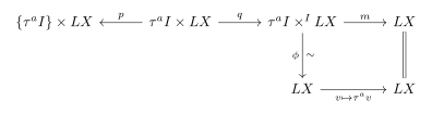
Figure 2. Convolution on the length-zero cell becomes translation via \(\phi([\tau^a i,v])=iv\). TikZ-cd source.
Here \(p(g,v)=(gI,v)\), \(q(g,v)=[g,v]\), and \(m([g,v])=gv\); descending \(p^*(\mathrm{IC}_{\tau^a}\boxtimes\mathrm{IC}_0)\) along \(q\) gives \(\phi^*\mathrm{IC}_0\), so convolution is \(m_!\phi^*\mathrm{IC}_0=(\tau^a)_!\mathrm{IC}_0\).
The convolution correspondence over the point \(\tau^aI\) is \(\tau^aI\times^I LX\cong LX\), with action map \(v\mapsto\tau^av\) (chain-stabilizer proof, convolution proof). The identification of length with cell dimension is [Zhu, Remark 2.1.22, p. 29]; the general length-zero subgroup and its Hecke algebra are described in [HKP, §7.1, p. 19]. Together with the first point and Proposition 4b, this gives generation by \(\{G_{\tau^a}:a\in\mathbb Z\}\).
The length-zero subgroup in Haines–Kottwitz–Prasad
For a split group, the extended affine Weyl group splits into its affine reflection group and the subgroup \(\Omega\) preserving the base alcove. In the characteristic-function normalization \(T_w=\mathbf1_{IwI}\), with \(\operatorname{vol}I=1\), its length-zero part is a group algebra:
Here \(W_{\mathrm{aff}}\) is generated by the affine simple reflections. HKP’s statement supplies these translation operators; reaching every simple support is the additional property of \(X=\mathbb A^n\) established above. [HKP, §7.1, p. 19]
For \(\mathrm{GL}_n\), determinant valuation gives \(\Omega=\langle\tau\rangle\cong\mathbb Z\). The identity \(\tau^n=t1_n\) makes \(\tau\) infinite order, although its action on the affine Dynkin diagram has order \(n\).
For \(G=\mathrm{GL}_n\), \(X=\mathbb A^n\), and the levels of §2, let \(\mathcal C_I\) be the category of §4. Use the one-step shift \(\tau\) constructed above, and put \(G_w=\mathrm{IC}_w\ast_I\mathrm{IC}_0\) for \(w\in\widetilde W\), the extended affine Weyl group. Then every simple \(S_a\) is obtained by translating the basic sheaf, up to shift:
Here \(S_a=\underline{\overline{\mathbb Q}}_{\ell,L_a}[-a]\) is the lattice-supported simple of Proposition 4a(b); \(\operatorname{Thick}\) allows shifts, cones and direct summands. The proof (§6) uses no traces and no (DT); taking traces recovers (IG) (§7). The variety \(\mathbb A^n\) has two \(G\)-orbits, so it is not a homogeneous symmetric variety and Chen–Yi does not apply.
1 · Objects
Definition 1.1 · Uniformizer and translations
Use \(k=\overline{\mathbb F}_q\), \(\mathcal O=k[\![t]\!]\), \(F=k(\!(t)\!)\), with their models over \(\mathbb F_q\) when taking traces.
Spaces and points. For an \(\mathbb F_q\)-algebra \(R\), the loop and arc functors are
$$LX(R)=R((t))^n,\qquad L^+X(R)=R[[t]]^n.$$
Thus \(F^n\) is the set of \(k\)-rational points of \(LX\); \(\mathbb F_q\)-rational loop points are \(LX(\mathbb F_q)=\mathbb F_q((t))^n\). Sheaves live on the geometric spaces, with their \(\mathbb F_q\)-models used for Frobenius traces.
Definition 1.2 · Extended affine Weyl group
For the diagonal torus \(T\subseteq\mathrm{GL}_n\),
$$\widetilde W=N_G(T)(F)/T(\mathcal O)\cong\mathbb Z^n\rtimes S_n.$$
Each class has a unique representative \(t^\lambda w\), with \(\lambda\in\mathbb Z^n\) and \(w\) a permutation matrix. The following map is a bijection:
$$\widetilde W\longrightarrow I(k)\backslash\mathrm{GL}_n(F)/I(k),\qquad t^\lambda w\longmapsto I(k)t^\lambda wI(k).$$
Let \(\varepsilon_i=(0,\ldots,0,1,0,\ldots,0)\in\mathbb Z^n=X_*(T)\), with \(1\) in position \(i\); in particular \(t^{\varepsilon_n}=\operatorname{diag}(1,\ldots,1,t)\). Let \(e_i\in F^n\) be the standard column vector, and let \(\sigma\) be the permutation matrix with \(\sigma e_1=e_n\), \(\sigma e_i=e_{i-1}\) for \(i>1\).
The standard action is matrix multiplication \(G\times X\to X\), \((g,v)\mapsto gv\). We choose its matrix
$$\tau=t^{\varepsilon_n}\sigma,\qquad \tau e_1=te_n,\quad\tau e_i=e_{i-1}\ (2\le i\le n),\qquad\tau^n=t\,1_n.$$
Here the displayed formulas describe the action on the basis vectors.
Normalization. The two reasons in the introduction use the following identities (proved in Weyl groups, Step 4):
$$\tau I\tau^{-1}=I,\qquad\ell(\tau)=0,\qquad\operatorname{val}\det\tau=1,\qquad\tau^k\mathcal O^n\supset\tau^{k+1}\mathcal O^n.$$
The length-zero subgroup is \(\Omega:=\{w\in\widetilde W:\ell(w)=0\}=\langle\tau\rangle\cong\mathbb Z\); \(\tau\) is its unique generator with determinant valuation \(+1\). The other generator, \(\tau^{-1}\), reverses the indexing. For \(n>1\), the plain cycle \(\sigma\) does not normalize \(I\); an arbitrary element of \(\widetilde W\) need not have length zero. Length zero makes convolution by \(\mathrm{IC}_{\tau^k}\) an actual translation (§6).
Example 1.4 · Action on vectors
How \(\tau\) acts. \(G=\mathrm{GL}_n\) acts on \(X=\mathbb A^n\) by matrix multiplication, so \(G(F)\) acts on \(LX(k)=X(F)=F^n\) by \(v\mapsto gv\); this is the only action on the page, and it also defines convolution (§6). \(\tau\in G(F)\) is one matrix, acting on column vectors by a cyclic shift with one factor \(t\):
$$\tau\begin{pmatrix}v_1\\ v_2\\ \vdots\\ v_n\end{pmatrix}=\begin{pmatrix}v_2\\ \vdots\\ v_n\\ t\,v_1\end{pmatrix},\qquad\tau^{-1}\begin{pmatrix}v_1\\ \vdots\\ v_{n-1}\\ v_n\end{pmatrix}=\begin{pmatrix}t^{-1}v_n\\ v_1\\ \vdots\\ v_{n-1}\end{pmatrix}.$$
Definition 1.5 · The periodic lattice chain
Geometric lattice convention. Write \(L_a:=\tau^aL^+X\subseteq LX\), so \(L_a(R)=\tau^aR[[t]]^n\) and \(L_a(k)=\tau^a\mathcal O^n\). In sheaf supports and geometric inverse images below, the notation \(\tau^a\mathcal O^n\) means \(L_a\), not merely its set of points.
Lattices. \(\mathcal O^n=L^+X(k)\) is a set of vectors, and \(\tau^k\mathcal O^n:=\{\tau^kv:v\in\mathcal O^n\}\) is its image under the linear map \(\tau^k\) (not \(\tau\) acting on the scalars). Applying \(\tau\) \(r\) times moves \(v_1,\dots,v_r\) to the end, each multiplied by \(t\); with \(\tau^n=t\cdot1_n\) and \(k=nm+r\), \(0\le r\lt n\):
$$\tau^k\mathcal O^n=t^m\big(\mathcal O^{\,n-r}\oplus(t\mathcal O)^{r}\big)=\{v:\ \operatorname{val}v_i\ge m\ (i\le n-r),\ \operatorname{val}v_i\ge m+1\ (i\gt n-r)\}.$$
It is \(I\)-stable, since \(\tau\) normalizes \(I\): \(I\tau^k\mathcal O^n=\tau^k(\tau^{-k}I\tau^k)\mathcal O^n=\tau^kI\mathcal O^n=\tau^k\mathcal O^n\). For \(n=2\): \(\tau(a,b)=(b,ta)\), so \(\tau\mathcal O^2=\mathcal O\oplus t\mathcal O\); \(\tau^2(a,b)=(ta,tb)\), so \(\tau^2\mathcal O^2=t\mathcal O^2\); \(\tau^{-1}(a,b)=(t^{-1}b,a)\), so \(\tau^{-1}\mathcal O^2=t^{-1}\mathcal O\oplus\mathcal O\). These are all the \(I\)-stable lattices (lattice lemma below): a decreasing chain \(\cdots\supset\tau^{-1}\mathcal O^n\supset\mathcal O^n\supset\tau\mathcal O^n\supset\cdots\), each of colength \(1\) in the previous one.
Choose the last coordinate attaining the minimum valuation. Upper-triangular operations modulo t and their congruence lifts carry the vector to the indicated coordinate vector; the valuation conditions identify its orbit with the displayed lattice difference. The linked orbit and lattice lemmas give the full elimination argument.
Lemma 1.10 · The periodic chain determines the Iwahori
Chain. \(\tau\Lambda_{m,j}=\Lambda_{m,j-1}\) on the \(\mathcal O\)-basis \(t^me_1,\dots,t^me_j,t^{m+1}e_{j+1},\dots\); with \(\Lambda_{0,n}=\mathcal O^n\) this gives \(\Lambda_{m,j}=\tau^{nm+n-j}\mathcal O^n\) (A5-1(a); script A5/lattice_checks.py (a), \(n\le5\)).
Normalizes. \(I\) is the stabilizer of the chain \(\{\Lambda_{m,j}\}\), which \(\tau\) permutes; so \(\tau I\tau^{-1}=I\), \(\ell(\tau)=0\) (A5-1(b)). Checked on all of \(I/I_{0,2}(\mathbb F_2)\) for \(n=2,3\), with the control that the plain cycle \(\sigma\) does not normalize \(I\) (script below, (6)).
2 · Levels \(Y_N\), \(Y_{N,M}\)
Set-up. For \(N,M\ge0\) with \(N+M\ge1\):
These are spaces and group schemes over \(\mathbb F_q\), specified for every \(\mathbb F_q\)-algebra \(R\) by
$$Y_N(R)=t^{-N}R[[t]]^n,\qquad Y_{N,M}(R)=t^{-N}R[[t]]^n/t^MR[[t]]^n,$$
$$I(R)=\{g\in\mathrm{GL}_n(R[[t]]):g\bmod t\in B(R)\},\qquad H_{N,M}(R)=\{g\in\mathrm{GL}_n(R[t]/t^{N+M}):g\bmod t\in B(R)\}.$$
The lattice formulas below give their \(k\)-points; the coefficient formulas define the schemes and their morphisms.
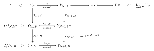
Figure 3. \(X=\mathbb A^n\), any \(n\): the levels of \(LX\), with \(LX(k)=F^n\), \(Y_N=t^{-N}\mathcal O^n\) and \(Y_{N,M}=t^{-N}\mathcal O^n/t^M\mathcal O^n\). Horizontal maps are closed embeddings, vertical maps are surjections, every square is cartesian, \(\pi_{N,M}=p_{M',M}\circ\pi_{N,M'}\) and \(Y_N=\varprojlim_MY_{N,M}\).
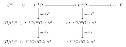
Figure 4. \(X=\mathbb A^1\) (\(n=1\)), \((N,M,M')=(1,1,2)\): the same diagram with \(LX(k)=F\); the vertical maps are reductions modulo \(t^2\) and \(t\).
Proposition 2 · One level
Let \(N,M\ge0\), \(N+M\ge1\), and write a point of \(Y_{N,M}\) as \(\sum_{a=-N}^{M-1}t^av_a\) with \(v_a\in\overline{\mathbb F}_q^{\,n}\). Then:
\(Y_{N,M}\cong\mathbb A^{n(N+M)}\), with coordinates \((v_{-N},\dots,v_{M-1})\).
\(I_{N,M}\) is the kernel of the action of \(I\) on \(Y_{N,M}\), and \(H_{N,M}\cong B\times\mathbb A^{n^2(N+M-1)}\) is connected of dimension \(n^2(N+M)-\binom n2\).
\(p_{M',M}\) forgets \(v_M,\dots,v_{M'-1}\): an equivariant trivial vector bundle of rank \(d(M,M')=n(M'-M)\). \(i_N\) identifies \(Y_N\) with the closed subspace \(\{v_{-N-1}=0\}\), and \(\pi_{N+1,M}^{-1}(Y_{N,M})=Y_N\).
The level shift of Proposition II (\(e_M=e_{M'}+d(M,M')\), \(e_0=0\)) is \(e_M=-nM\), and \(\Phi_{N,M}=i_{N,!}\pi_{N,M}^*[e_M]\) sends perverse sheaves to perverse objects.
(b) Trivial action. \((1+t^{N+M}A)v-v\in t^{N+M}\cdot t^{-N}\mathcal O^n=t^M\mathcal O^n\). Conversely \(g\,t^{-N}e_i\equiv t^{-N}e_i\bmod t^M\) for all \(i\) forces \(g-1\in t^{N+M}M_n(\mathcal O)\): \(I_{N,M}\) is the whole kernel (checked: only \(g=1\) in \((I/I_{N,M})(\mathbb F_q)\) acts trivially, every case of the script).
(b) Connected. \(H_{N,M}\) is the open subset \(\{g_{aa}(0)\ne0\}\) of the affine space of truncated matrices with \(g_{ab}(0)=0\) for \(a\gt b\): irreducible. \(I_{N,M}\subseteq1+tM_n(\mathcal O)\) is pro-unipotent because \(N+M\ge1\) (at \(N=M=0\) the formula would leave \(I\)).
(c) Transitions. \(Y_{N,M'}\to Y_{N,M}\) forgets \(v_M,\dots,v_{M'-1}\): a trivial vector bundle of rank \(n(M'-M)\), equivariant for \(I/I_{N,M'}\to I/I_{N,M}\), with rank independent of \(N\). \(Y_N\subset Y_{N+1}\) is \(\{v_{-N-1}=0\}\), and \(\pi_{N+1,M}^{-1}(Y_{N,M})=t^{-N}\mathcal O^n+t^M\mathcal O^n=Y_N\) for every \(M\ge0\).
(d) Shift. With \(\Phi_{N,M}=i_{N,!}\pi_{N,M}^*[e_M]\) and \(p:Y_{N,M'}\to Y_{N,M}\), \(p^*[d(M,M')]\) is t-exact, and \(\Phi_{N,M}=\Phi_{N,M'}\circ p^*[d(M,M')]\) iff \(e_M=e_{M'}+d(M,M')\) (the shift \(e_M\)). With \(d(M,M')=n(M'-M)\) and \(e_0=0\): \(e_M=-nM\), and \(\Phi_{N,M}(K)\) is perverse iff \(K\) is perverse on \(Y_{N,M}\) (A5-2).
3 · Geometric inputs used below
Fix \(N,M\ge0\), \(N+M\ge1\), and put \(L_a=\tau^aL^+X\), \(H=H_{N,M}\); all geometric statements are over \(k=\overline{\mathbb F}_q\).
Proposition 3a · Strata, closures, and stabilizers
Finite orbit stratification. The \(H\)-orbits on \(Y_{N,M}\) are
$$Y_{N,M}=\bigsqcup_{a=-nN}^{nM}o_a,$$
$$o_a=V_a\setminus V_{a+1}\quad(a<nM),$$
$$o_{nM}=V_{nM}=\{0\},$$
where \(V_a=L_a/L_{nM}=\tau^a\mathcal O^n/t^M\mathcal O^n\).
Used in Proposition 4a(a) to locate the supports of simple objects.
Smooth linear closures. For \(-nN\le a\le nM\),
$$\overline{o_a}=V_a\cong\mathbb A^{nM-a},$$
$$V_{-nN}\supset V_{-nN+1}\supset\cdots\supset V_{nM},$$
$$\pi_{N,M}^{-1}(V_a)=L_a,$$
$$P_a:=\pi_{N,M}^{-1}(o_a)=L_a\setminus L_{a+1}\quad(a<nM),$$
$$P_{nM}=L_{nM}.$$
Used in Proposition 4a(a),(b) to compute the IC complexes and their pullbacks, and in Proposition 7 to expand traces in piece indicators.
Smooth connected stabilizers. For \(-nN\le a=nm+n-j<nM\), \(1\le j\le n\), the orbit \(o_a\) contains \(t^me_j\), and
$$\operatorname{Stab}_H(t^me_j)=\{g\in H:g_{ij}\equiv\delta_{ij}\pmod{t^{M-m}}\ \text{for every }i\}\cong\mathbb G_m^{n-1}\times\mathbb A^{b_a},$$
as varieties, for some \(b_a\ge0\); \(\operatorname{Stab}_H(0)=H\) is also smooth connected.
Used in Proposition 4a(a): the only irreducible equivariant local system on each orbit is the constant rank-one system.
Let \(N,M\ge0\), \(N+M\ge1\), and \(V_a\) be the linear closures in Proposition 3a. Constant sheaves on closed supports below are extended by zero.
One level. The simple \(H_{N,M}\)-equivariant perverse sheaves on \(Y_{N,M}\) are exactly
$$\mathrm{IC}(V_a)=\underline{\overline{\mathbb Q}}_{\ell,V_a}[nM-a],\qquad-nN\le a\le nM .$$
The objects \(S_a\). Their normalized images are independent of the level containing them:
$$S_a:=\Phi_{N,M}\big(\mathrm{IC}(V_a)\big)=\underline{\overline{\mathbb Q}}_{\ell,L_a}[-a].$$
$$S_0=\mathrm{IC}_0.$$
These are all the simple objects in the perverse heart of \(\mathcal C_I\).
Translation. For every \(a\in\mathbb Z\),
$$S_a=(\tau^a)_!\mathrm{IC}_0[-a],\qquad (\tau^a):LX\xrightarrow{\sim}LX,\quad v\longmapsto\tau^av .$$
Proof
Classify at one level. The finite orbit stratification in Proposition 3a(a) makes every simple an IC extension from an irreducible equivariant local system on one \(o_a\) (BBD, Theorem 4.3.1, printed p. 112). Such local systems correspond to representations of the stabilizer component group; this group is trivial by Proposition 3a(c). Thus there is exactly one simple per orbit. Since \(\overline{o_a}=V_a\) is smooth of dimension \(nM-a\) (Proposition 3a(b)), that simple is \(\underline{\overline{\mathbb Q}}_{\ell,V_a}[nM-a]\).
Compute the normalized image. By Proposition 3a(b) and \(e_M=-nM\),
$$\begin{aligned}\Phi_{N,M}\big(\mathrm{IC}(V_a)\big)&=i_{N,!}\pi_{N,M}^*\underline{\overline{\mathbb Q}}_{\ell,V_a}[nM-a-nM]\\&=\underline{\overline{\mathbb Q}}_{\ell,L_a}[-a].\end{aligned}$$
The normalized transition functors identify these objects at common refinements and preserve simples; Lemma IIa, steps 4–7 proves this compatibility, and step 8 proves that every global simple occurs at a finite level. This proves (b), including \(S_0=\mathrm{IC}_0\).
Translate the support. The automorphism \(v\mapsto\tau^av\) carries \(L_0\) isomorphically onto \(L_a\), hence
$$(\tau^a)_!\mathrm{IC}_0=\underline{\overline{\mathbb Q}}_{\ell,L_a}=S_a[a].$$
It preserves \(I\)-equivariance because \(\tau^a\) normalizes \(I\) (Lemma 1.10).
Sources
Reading Proposition 4a(b). \(\underline{\overline{\mathbb Q}}_{\ell,\tau^k\mathcal O^n}[-k]\) is shorthand for an object built at a finite level:
Object. \(\mathrm{IC}(V_k)\) is the constant sheaf on the linear subspace \(V_k\subseteq Y_{N,M}\cong\mathbb A^{n(N+M)}\), shifted by \(\dim V_k\); \(S_k\) is its pull-back to \(Y_N\), extended by zero to \(LX\).
Support. \(\pi_{N,M}^{-1}(V_k)=\tau^k\mathcal O^n\) (Definition 1.5): the stalks of \(S_k\) are \(\overline{\mathbb Q}_\ell[-k]\) on \(\tau^k\mathcal O^n\) and \(0\) off it.
Shift. \(-k=\dim V_k+e_M=(nM-k)-nM\), the perverse degree \(\delta(P_k)\), independent of \((N,M)\).
Here \(\operatorname{Thick}\) allows finite sums, shifts, cones and direct summands; no semisimplicity is asserted.
The level window is \(L_{nM}\subseteq L_a\subseteq L_{-nN}\iff-nN\le a\le nM\). The zero-orbit skyscraper at level \((N,M)\) pulls back to \(S_{nM}=\underline{\overline{\mathbb Q}}_{\ell,t^M\mathcal O^n}[-nM]\); the singleton \(\{0\}\subset LX\) is not a union of fibres of any fixed \(\pi_{N,M}\).
Proof
Build perverse objects from simples. Write \(\mathcal D_{N,M}=D^b_c([Y_{N,M}/H_{N,M}])\). Its equivariant perverse heart has finite length (BBD, Theorem 4.3.1; Lemma IIa, step 6). A Jordan–Hölder filtration of any perverse object has quotients among the \(\mathrm{IC}(V_a)\) of Proposition 4a(a); each short exact sequence gives a distinguished triangle. Thus every perverse object lies in their thick span.
Build bounded complexes from cohomology. For \(K\in\mathcal D_{N,M}\), the perverse t-structure is bounded, and its truncation triangles are
$${}^p\tau_{\le j-1}K\longrightarrow{}^p\tau_{\le j}K\longrightarrow{}^pH^j(K)[-j]\xrightarrow{+1}.$$
Only finitely many \({}^pH^j(K)\) are nonzero. Step 1 and induction through these triangles give
$$\mathcal D_{N,M}=\operatorname{Thick}\{\mathrm{IC}(V_a):-nN\le a\le nM\}.$$
This is the finite-length and truncation argument of Lemma IIa, step 8.
Pass through the level functors. The exact fully faithful functor \(\Phi_{N,M}\) sends these generators to \(S_a\) by Proposition 4a(b). Its essential image is closed under direct summands, since a bounded t-structure implies idempotent completeness ([CD, Proposition B.2.1, p. 109]); hence the finite-level equality follows. Every object of \(\mathcal C_I\) lies at a finite level, while every integer \(a\) lies in a window \([-nN,nM]\). A finite collection of such windows admits a common refinement, so the directed union gives the second equality.
Sources
BBD supplies finite length; the truncation and level arguments are given above and in Lemma IIa. The Stacks extracts supply the conventions for thick closure.
6 · Proof
Goal. \(G_{\tau^k}=S_k[k]\) and \(\mathcal C_I=\operatorname{Thick}\{G_{\tau^k}\}\), from §1, Proposition 4a and Proposition 4b.
Find the length-zero kernels
For a length-zero element the Schubert variety is a point and its IC sheaf a skyscraper:
Convolution. As in Proposition II, \(\mathcal G\ast_IM=m_!(\mathcal G\mathbin{\widetilde\boxtimes}M)\), where
$$LG\times^ILX=(LG\times LX)/I,\ \ (g,x)\sim(gi,i^{-1}x),\qquad m[g,x]=gx,\qquad\mathrm{pr}[g,x]=gI\in\mathrm{Fl},$$
and \(\mathcal G\mathbin{\widetilde\boxtimes}M\) is the descent of \(\mathcal G\boxtimes M\) from \(LG\times LX\), which exists because \(M\) is \(I\)-equivariant. There is no normalizing shift.
Support. \(\delta_{\tau^k}\) is \(\overline{\mathbb Q}_\ell\) in degree \(0\) at the point \(\tau^kI\), an object of the Hecke category because the point is \(I\)-fixed (step 1). So \(\delta_{\tau^k}\mathbin{\widetilde\boxtimes}M\) lives on the fibre \(\mathrm{pr}^{-1}(\tau^kI)=\tau^kI\times^ILX\).
The fibre is \(LX\). \(j:LX\xrightarrow{\sim}\tau^kI\times^ILX\), \(y\mapsto[\tau^k,y]\), with inverse \([\tau^ki,x]\mapsto ix\) (well defined: \([\tau^kii',i'^{-1}x]\mapsto ix\)). Under \(j\), \(\delta_{\tau^k}\mathbin{\widetilde\boxtimes}M\) is \(M\).
Action. \(m(j(y))=\tau^ky\), so \(\delta_{\tau^k}\ast_IM=(m\circ j)_!M=(\tau^k)_!M\), which is \(I\)-equivariant because \(\tau^{-k}I\tau^k=I\). With \(M=\mathrm{IC}_0\), Proposition 4a(c) gives \(S_k[k]\) (A5-3(a), audit A8-9).
Literature. The same mechanism as Bezrukavnikov–Yun, Lemma 3.2.2: when lengths add, \(m\) restricts to an isomorphism, here with \(\ell(\tau^k)=0\). At the level of functions it is [HKP, Lemma 7.2.1(iii)]: \(T_\tau\) acts by translation. Chen–Yi use the same convolution \(a_!(M\mathbin{\widetilde\boxtimes}F)\) (proof of Proposition 70).
\(n=1\) (\(\tau=t\)): \(\mathrm{Fl}=F^\times/\mathcal O^\times=\mathbb Z\) is discrete, every \(\mathrm{IC}_{t^k}=\delta_{t^k}\), and \(G_{t^k}=\underline{\overline{\mathbb Q}}_{\ell,t^k\mathcal O}=S_k[k]\): these are all the generators.
Why \(\tau^k\). The \(w\in\widetilde W\) with \(w\mathcal O^n=\tau^k\mathcal O^n\) are the \(w=\tau^ku\), \(u\in S_n=\widetilde W\cap K\). Lengths add, so \(\Delta_w=\delta_{\tau^k}\ast_I\Delta_u\) (\(\Delta_u\) the constant sheaf on \(IuI/I\cong\mathbb A^{\ell(u)}\), extended by zero), and \(IuI\subseteq K\) fixes \(\mathcal O^n\), so \(\Delta_w\ast_I\mathrm{IC}_0=G_{\tau^k}\otimes H^*_c(\mathbb A^{\ell(u)})=G_{\tau^k}[-2\ell(u)](-\ell(u))\): the same object, shifted. \(\tau^k\) is the shortest choice. For example \(t^{(0,1)}=\tau s_1\) for \(n=2\).
Sources
Close under shifts
Every simple object is a shifted generator, and the simple objects generate:
Proposition 4b and step 2; a thick subcategory is closed under shifts. Last inclusion: every \(G_w\) lies at level \((c,c)\), \(c=c(w)\), by (Dict)(d) with \(N=M=0\). The other generators, such as \(G_{s_0}\), are not needed.
7 · The classical statement
Here all functions are on rational points: \(F_0=\mathbb F_q((t))\), \(\mathcal O_0=\mathbb F_q[[t]]\), \(I_0=I(\mathbb F_q)\), and \(C_I=C_c^\infty(F_0^n)^{I_0}\). The trace of a sheaf is evaluated at its \(\mathbb F_q\)-rational points.
A constant sheaf has trace \(1\) on its support and \(\operatorname{tr}(K[1])=-\operatorname{tr}K\) (trace additivity in IIb); \(\tau^k\mathcal O_0^n=\bigsqcup_{k'\ge k}P_{k'}(\mathbb F_q)\) by Proposition 3a(a),(b). So the matrix to the piece indicators is upper triangular with every entry of row \(k\) on or above the diagonal equal to \((-1)^k\) (script (7)).
Sources
Corollary · (IG) for 𝔸ⁿ
Let \(T_w=\mathbf 1_{I_0wI_0}\in\mathcal H_I\) (\(\operatorname{vol}I_0=1\)) and \(\varphi_0=\mathbf 1_{\mathcal O_0^n}\in C_I\). Then
the direct function calculation(a) computes \(T_{\tau^k}\ast\varphi_0=\mathbf 1_{\tau^k\mathcal O_0^n}\) directly from \(I\tau^kI=\tau^kI\); here it is read off from the sheaves of §6.
Take traces of generators
The trace of a length-zero generator is a translate of \(\varphi_0\):
First equality: trace of a convolution, with \(\operatorname{tr}\delta_{\tau^k}=T_{\tau^k}\) and \(\operatorname{tr}\mathrm{IC}_0=\varphi_0\) (Lemma IIb). Then §6, step 2 and Proposition 7.
Proof
\(\tau^k\in\mathrm{GL}_n(\mathbb F_q(\!(t)\!))\), so the isomorphism of §6, step 2 is defined over \(\mathbb F_q\), with Frobenius acting by \(1\) on the stalks \(\overline{\mathbb Q}_\ell\) of \(\mathrm{IC}_0\).
\(n=2\), not length zero: \(G_{s_0}=S_{-1}\oplus S_1\) (A5-3(c)), and with \(\operatorname{tr}\mathrm{IC}_{s_0}=-(T_e+T_{s_0})\),
$$\operatorname{tr}G_{s_0}=-(\varphi_0+T_{s_0}\ast\varphi_0)=-\mathbf 1_{\tau^{-1}\mathcal O_0^2}-q\,\mathbf 1_{\tau\mathcal O_0^2}=\operatorname{tr}S_{-1}+q\operatorname{tr}S_1 .$$
So a generator's trace can have coefficient \(q\) on \(\operatorname{tr}S_k\); the length-zero ones have a single coefficient \(\pm1\).
Sources
Span the functions
At each level the traces of the simple objects are a basis, so the generator traces span \(C_I\):
The \(\mathbf 1_{P_k(\mathbb F_q)}\) are a basis (Proposition 3b, step 3 of Proposition II), the \(\operatorname{tr}S_k\) are triangular in them with diagonal \(\pm1\) (Proposition 7), then step 1. Take the union over \((N,M)\).
This uses that every simple object is a shifted generator. Thick generation alone would not give it: \(\operatorname{Thick}\) is closed under direct summands, and \([A]\notin\mathbb Z[A\oplus B]\) in the Grothendieck group.
8 · Hypotheses of Proposition II
Table 4. Each hypothesis of Proposition II for \(\mathbb A^n\); §6 uses only (Lev), I1, I2 and (Dict)(d).
hypothesis
for \(\mathbb A^n\)
where
(Lev)
linear projections with fibre \(\mathbb A^{n(M'-M)}\); \(Y_N=\{v_{-N-1}=0\}\subset Y_{N+1}\); \(I/I_{N,M}\cong B\times\mathbb A^{n^2(N+M-1)}\) connected, \(I_{N,M}\) pro-unipotent; \(\pi_{N,M}^*\) fully faithful
With \(F_0=\mathbb F_q((t))\), \(\mathcal O_0=\mathbb F_q[[t]]\): \(Y_N(\mathbb F_q)=t^{-N}\mathcal O_0^n\) is compact open; \(\bigcup_NY_N(\mathbb F_q)=F_0^n\), and cosets of \(t^M\mathcal O_0^n\) form a basis
—
(Dict)(c)
\(o_k=V_k\setminus V_{k+1}\) is defined over \(\mathbb F_q\) and contains \(t^me_j\)
(Dict)(d). \(\overline{IwI}=\bigsqcup_{v\le w}IvI\) is compact, so some \(c=c(w)\ge0\) has \(g,g^{-1}\in t^{-c}M_n(\mathcal O)\) on it. Then \(gY_N\subseteq Y_{N+c}\), and \(x\equiv x'\bmod t^{M+c}\) gives \(g^{-1}x\equiv g^{-1}x'\bmod t^M\). For \(n=1\), \(w=\tau^k=t^k\): \(c=|k|\).