In June we drive out of Rome to the Gran Sasso, and end in the stone village of Santo Stefano di Sessanio.
The hard part of a mountain plan is not the walking. It is deciding, honestly, what the mountain will allow.
So I keep two plans side by side. One is ambitious: sleep high at the huts, cross Corno Grande, traverse the ridge.
The other is safer: a car between trailheads, the same views, none of the commitments I cannot keep.
The unknowns choose between them — whether the huts have really opened, and how much snow stays on the high traverses in late June.
Full itinerary, decision gates, and the route-risk matrix:
Gran Sasso High Route Plan — June 14–18, 2026.

It is ironic always. We only perceive symmetry.
Yet, we are governed by symmetry.
That the most beautiful things in the world appear seemingly symmetric.
Like the Kepler snowflake.
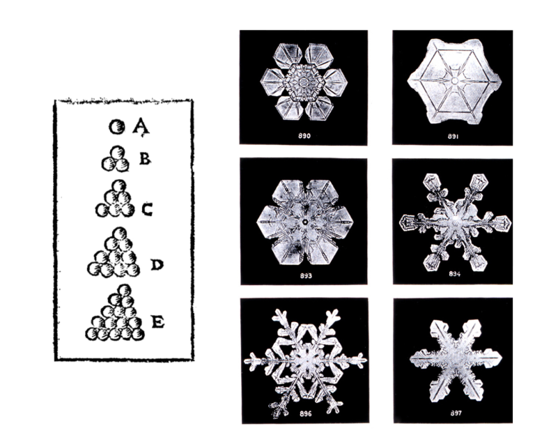
This symmetry is perceived.
Large, inanimate aggregates of matter find it favorable to settle, to choose a side, to become anisotropic.
In the macroscopic limit, the "fair" symmetry is sacrificed for the rigidity.
It is, however, governed by symmetry.
The physical world is governed by physical laws, which are translational and rotational invariance.
Similarly, humans have underlying laws of what they desire in love.
This is called "harmony" in a daily sense.
Love does not have this symmetry.
It is this part of nature that I never accept.
The goal of love appears as a harmony.
Yet, it is a broken symmetry.1
1 Anderson, P. W. (1972). More Is Different. Science, 177(4047), 393–396. [pdf]
The word "consolidate" comes from two Latin roots.
Com-: to gather together. Solidare: to make solid.
To consolidate is therefore both to add and to rigidify.
But what is taken away? I think when we learn we always take away.
The word "consolidate" comes from two Latin roots.
Com-: to gather together. Solidare: to make solid.
To consolidate is therefore both to add and to rigidify.
Supposedly then, to make solid, is the act of protecting what is already there.
What is strengthened is unclear to me.
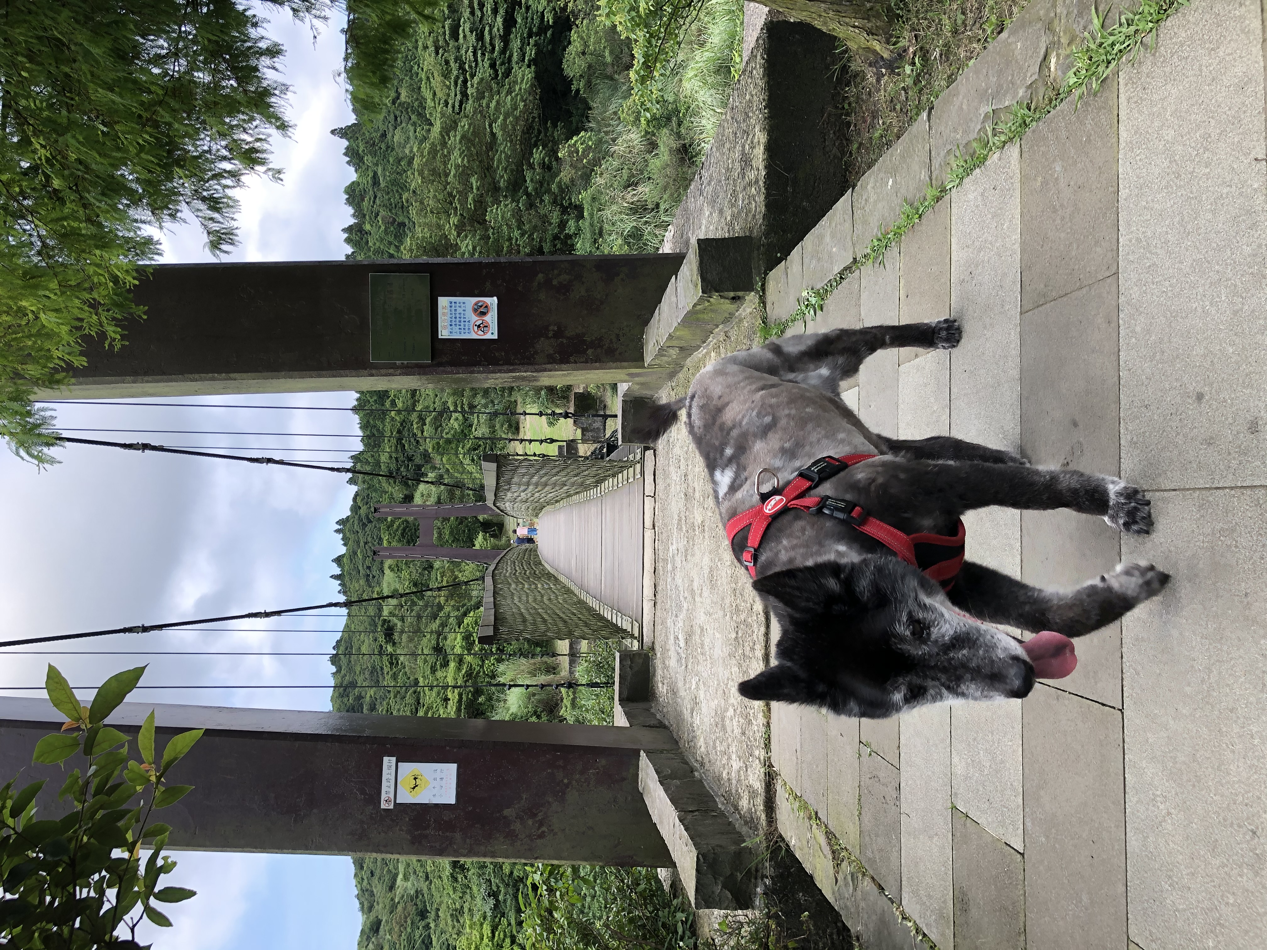
If you ask me to recall my home, the mountain I spent half of my life,
I don't remember a single thing. All I remember are just the colors.

The silver grass that is more gold than silver in Autumn days.
And also the friends, and the loved ones, that I shared those colors with.
I wanted to go for the "big dreams."
I had only one graduate school, so of course I had to go for a problem.
I was rather proud of myself for doing a problem in the Langlands program, coming into the fourth year of my PhD.
Then the dream scales down. In what sense?
I felt that it is perhaps only a dream. A dream that I imagined and not meant to be close to what I think reality is.
There was an intrinsic human element missing from this dream.
Deep behind my back, I was no longer sure if these are "dreams" of what I want.
I was jumping between areas, or as my friend Naruki says, I have the shiny object problem.
When it comes to practice, mathematics is long.
I had the good fortune to collaborate with various mathematicians.
The "proof process" I have so much enjoyed has become mundane.
Why? It is a cycle of idea generation, literature review, execution.
The particular part of execution has become a constant.
This part might change within the foreseeable future of AI.
With our personal robot avatars:
![]()
There are plenty who are smarter than me.
Some may say the process is the most important in mathematics.
But maybe not when it repeats.
Graduating this year. What next? I like new phenomena.
If I had done maths again, I wish I had attempted to explore some new phenomena.
But this isn't so clear all the time as what count as a "good" phenomenon.
There was also the realistic pressure of coming up with ideas with something cohesive and plausible.
Do I have time? What exactly am I good at?
If the academic system allows the flexibility to jump beyond different areas, relearn, re-explore, collaborate, and teach, then that would be great.
To some extent, I think there is a matter of "parallel thinking" in research.
How could you identify ideas that are parallel?
Things you could do at the same time.
Much of it requires identifying the "necessary steps" before the branching factor increases.
The ability to identify this necessary step is slightly harder.
The core object in memory should not be "conversation."
It should be a research node with fields: question, node type, dependencies, evidence needed, expected signature, evaluator, cost, stop rule, unlocks, and current confidence, blah, blah... but so then is this a good idea?
This makes the system reason over a graph of epistemic dependencies rather than over a flat chat history.
On characters
But yet, what are characters? They have various definitions — see §1. But where do roots come from? — see §2. Then we might want to see how they are used in representation theory — see §3. The terminology is loaded: the word “character” refers to at least three different objects, and the punchline is that weights of a representation are characters of the maximal torus that occur in it. A small running example ($SL_2$ acting on $\mathbf{C}^2$) is worked out in detail in SL$_2$ moment map and the conormal of $B\cdot(1,0)$.
§1. Three meanings of “character”
Fix a (split) reductive group $G$ over a field, a split maximal torus $T\subset G$ with character lattice $X^*(T) = \operatorname{Hom}(T,\mathbb{G}_m)$, and a finite-dimensional representation $\rho : G \to \mathrm{GL}(V)$. Three different objects in the literature get called “character”:
| name | object | notation |
|---|---|---|
| algebraic group character | algebraic group homomorphism $G \to \mathbb{G}_m$ | $\chi : G \to \mathbb{G}_m$ |
| representation (trace) character | conjugation-invariant function $g \mapsto \mathrm{Tr}(\rho(g))$ | $\Theta_V(g) = \mathrm{Tr}(\rho(g))$ |
| formal character | weight-multiplicity record in $\mathbb{Z}[X^*(T)]$ | $\operatorname{ch}_T(V) = \sum_\lambda m_\lambda\, e^\lambda$ |
These are not the same object. An algebraic group character is a homomorphism; the trace character $\Theta_V$ is in general not multiplicative, only a conjugation-invariant class function on $G$. I will write $\Theta_V$ for the trace, so that it is not confused with an algebraic group character $\chi : G \to \mathbb{G}_m$. The formal character $\operatorname{ch}_T(V)$ is a bookkeeping device living in the group ring of the character lattice, and the Weyl character formula is an identity inside $\mathbb{Z}[X^*(T)]$.
§2. Where do roots come from?
Start with a split reductive group $G$, a split maximal torus $T\subset G$, and the Lie algebra $\mathfrak g$. The torus $T$ acts on $\mathfrak g$ by the adjoint action, $$ T \curvearrowright \mathfrak g, \qquad t\cdot X \;=\; \mathrm{Ad}(t)\,X. $$ Representations of a split torus are completely reducible into character eigenspaces, so $\mathfrak g$ decomposes as a direct sum of $X^*(T)$-graded pieces. A root is a nonzero character $$ \alpha : T \longrightarrow \mathbb{G}_m $$ such that $T$ acts on some nonzero line $\mathfrak g_\alpha \subset \mathfrak g$ by the rule $$ t\cdot X \;=\; \alpha(t)\,X. $$ Write $\Phi\subset X^*(T)\setminus\{0\}$ for the set of roots. Then:
$\mathfrak g \;=\; \mathfrak t \;\oplus\; \bigoplus_{\alpha\in\Phi}\mathfrak g_\alpha.$
Roots are the “frequencies” with which $T$ acts on the non-torus directions of $G$. Equivalently, they are the nontrivial weights of the adjoint representation. The whole moment-map / cotangent picture in the $SL_2$ example rests on exactly this: the torus eats up the rest of $\mathfrak g$ via its characters.
§3. Characters versus weights
Now suppose $G$ is a reductive group and $\rho : G \to \mathrm{GL}(V)$ is a finite-dimensional representation. Choose a maximal torus $T\subset G$ and restrict $\rho$ to $T$: $$ \rho|_T \;:\; T \longrightarrow \mathrm{GL}(V). $$ Representations of a split torus are completely reducible into character eigenspaces, so $$ V \;=\; \bigoplus_{\lambda\in X^*(T)} V_\lambda, \qquad V_\lambda \;=\; \{\,v\in V \,:\, t\cdot v = \lambda(t)\,v\ \text{for all}\ t\in T\,\}. $$ The $\lambda\in X^*(T)$ for which $V_\lambda\neq 0$ are called the weights of $V$. Conrad states this as the equivalence between representations of a torus $T$ and $X^*(T)$-graded vector spaces.
The trace character of $V$, restricted to $T$, then decomposes as $$ \Theta_V|_T \;=\; \sum_{\lambda\in X^*(T)} \dim(V_\lambda)\, e^\lambda \;=\; \operatorname{ch}_T(V) \;\in\; \mathbb{Z}[X^*(T)], $$ where $e^\lambda$ is a formal exponential recording the weight $\lambda$. This is precisely the identity in which the Weyl character formula lives.
Weights are characters of the maximal torus that occur in a representation.
Roots are the weights of the adjoint representation $\mathfrak g$ (excluding $0$).
cf. Conrad, Reductive group schemes notes — weight-space decomposition for split tori, algebraic-group form of the Weyl character formula, and the identity $\Theta_V|_T = \sum_\mu \dim V(\mu)\, t^\mu$ inside $\mathbb{Z}[X^*(T)]$. For a concrete worked example with $G = SL_2$ and $V = \mathbf{C}^2$, where the $B$-action and its weights drive a cotangent / moment-map computation, see SL$_2$ moment map and the conormal of $B\cdot(1,0)$ (background on the $B$-action and its weights: S1; symplectic background: F1).
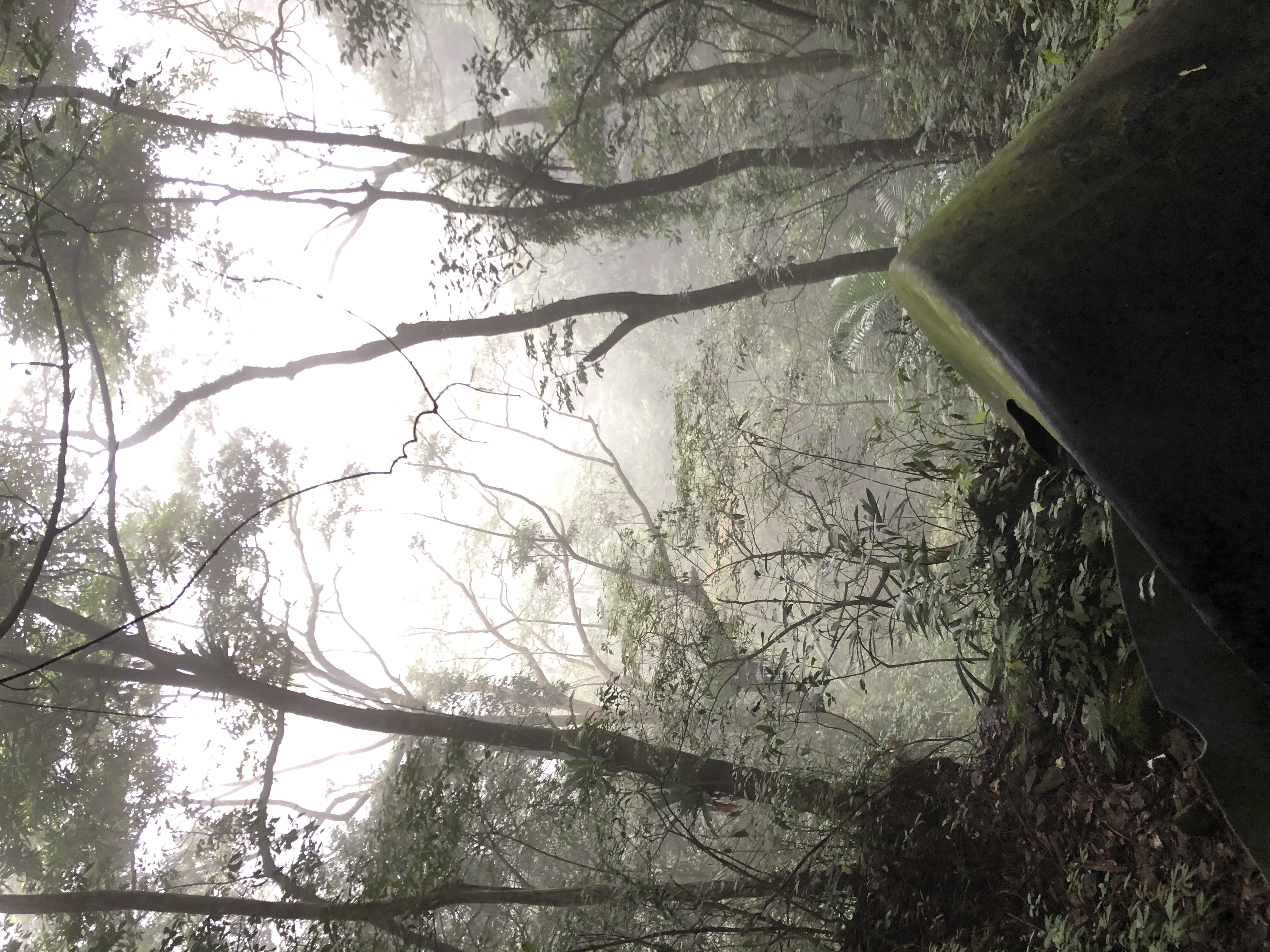
I think the rain reminds me of many things. the first things are the seasonal typhoons. Typhoons always gave me a sense of calmness.
I like the white mountain.

I think these ideas are quite applicable… even for mathematicians.
Why linear temporal logic? It is the vocabulary for properties of infinite executions — reactive systems (servers, controllers, protocols) that are never meant to halt.
§1. Syntax (BNF)
The set of formulas $\Phi$ is generated by the grammar
$$\varphi ::= \text{true} \mid a \mid \varphi_1 \wedge \varphi_2 \mid \neg\varphi \mid \bigcirc\varphi \mid \varphi_1 \, \mathsf{U} \, \varphi_2$$This is written in Backus–Naur form (Backus & Naur, ALGOL 60): $::=$ reads "is defined as" and $\mid$ reads "or". So a formula is built from $\text{true}$, an atomic proposition $a \in AP$, conjunction, negation, Next $\bigcirc$, and Until $\mathsf{U}$. Here $AP$ is the set of atomic propositions — the indivisible boolean facts that are true or false at a single step (e.g. for a traffic light, $\{\textsf{red}, \textsf{yellow}, \textsf{green}\}$).
§2. Temporal operators (semantics)
Fix the model. A trace is an infinite word $\sigma = \sigma_0\sigma_1\sigma_2\cdots \in (2^{AP})^{\omega}$, where $\sigma_i \subseteq AP$ is the set of propositions holding at step $i$. Satisfaction is a relation
$$\models \;\subseteq\; (2^{AP})^{\omega}\times\mathbb{N}\times\Phi, \qquad \sigma,i \models \varphi \;\;\text{("$\varphi$ holds at position $i$")}.$$The symbol $\models$ is the satisfaction relation: $\sigma,i \models \varphi$ reads "standing at step $i$ of trace $\sigma$, the formula $\varphi$ is true" — it is the bridge from syntax (the formula) to the trace (the system's reality). The two temporal operators are then:
$$\boxed{\;\sigma,i \models \bigcirc\varphi \iff \sigma,\,i+1 \models \varphi\;}$$ $$\boxed{\;\sigma,i \models \varphi_1\,\mathsf{U}\,\varphi_2 \iff \exists\, j\ge i:\ \sigma,j\models\varphi_2 \ \text{ and }\ \forall\, k,\ i\le k§3. Derived operators
From this grammar one recovers the rest of the standard vocabulary:
- $\Diamond\varphi \equiv \text{true}\,\mathsf{U}\,\varphi$ — "eventually": $\exists j\ge i.\ \sigma,j\models\varphi$.
- $\Box\varphi \equiv \neg\Diamond\neg\varphi$ — "always": $\forall j\ge i.\ \sigma,j\models\varphi$.

The smell of decay.
The optimal denoiser is the statistical center of gravity
A clean signal $X\in\mathbb R^d$ is corrupted into a noisy observation $Y\in\mathbb R^d$, and we want a rule $f$ that maps $Y$ back to a guess for $X$. Under squared-error loss the best possible rule is the posterior mean $f^\star(y)=\mathbb E[X\mid Y=y]$ — and that is exactly the center of mass of the posterior distribution $P(X\mid y)$. The whole story is one sentence: the optimal denoiser is the statistical center of gravity of your noisy observation.
§1. The problem
Let $X\in\mathbb R^d$ be the clean signal and $Y\in\mathbb R^d$ the observation. A denoiser is any measurable map $f:\mathbb R^d\to\mathbb R^d$, scored by its mean squared error
$$\mathcal R(f)=\mathbb E_{X,Y}\!\left[\,\|X-f(Y)\|^2\,\right].$$If $f^\star$ minimizes $\mathcal R$, what is the value $f^\star(y)$ at a given observation $y$? Write $D^\star(y)$ for the optimal pointwise guess. The answer is the posterior mean:
$f^\star(y)\;=\;D^\star(y)\;=\;\mathbb E[X\mid Y=y]\;=\;\operatorname*{arg\,min}_{a\in\mathbb R^d}\ \mathbb E\!\left[\,\|X-a\|^2\,\middle|\,Y=y\right].$
Three things are worth separating: why the global problem reduces to this pointwise one (§2), the physical picture that makes the answer obvious (§3), and the formal proof (§4). A visualization closes the note (§5).
§2. Why the global optimum is pointwise
By the law of total expectation, the global risk splits into an inner average over $X$ given a fixed observation and an outer average over observations:
$$\mathcal R(f)=\mathbb E_Y\!\left[\,\mathbb E_{X\mid Y}\!\left[\|X-f(Y)\|^2\,\middle|\,Y=y\right]\right] =\int\Big(\mathbb E\!\left[\|X-f(y)\|^2\,\middle|\,Y=y\right]\Big)\,p(y)\,dy.$$The weight $p(y)\ge 0$ and the inner term is a squared distance, hence $\ge 0$. To make the integral as small as possible there is no choice but to minimize the inner bracket separately for every $y$. For a fixed $y$ the output $f(y)$ is just some vector $a$, so $D^\star(y)$ must solve $\operatorname*{arg\,min}_a \mathbb E[\|X-a\|^2\mid Y=y]$, and therefore $D^\star(y)=f^\star(y)$.
Global optimality $\Rightarrow$ local optimality: the best function is the one that makes the best possible guess at every single observation.
§3. Moment of inertia and the parallel-axis theorem
The pointwise problem is literally a mechanics problem. In physics the moment of inertia of a mass density $\rho$ about an axis $a$ is
$$I_a=\int \|x-a\|^2\,\rho(x)\,dx.$$Take $\rho(x)=P(x\mid y)$, the posterior treated as a physical mass. Then $I_a=\mathbb E[\|X-a\|^2\mid Y=y]$ is exactly the expected squared error we want to minimize: we are looking for the axis that the posterior mass is “easiest to spin” about. The parallel-axis theorem answers it in one line,
$$I_a=I_{\mathrm{cm}}+M\,\|a-x_{\mathrm{cm}}\|^2,\qquad x_{\mathrm{cm}}=\int x\,\rho(x)\,dx=\mathbb E[X\mid Y=y],\qquad M=\!\int\!\rho=1.$$Here $I_{\mathrm{cm}}$ is a fixed property of the mass — the irreducible posterior variance, the Bayes error you cannot remove — and the total mass is $M=1$. The only term you control is the distance $\|a-x_{\mathrm{cm}}\|^2$, minimized uniquely by driving the axis through the center of mass, $a=x_{\mathrm{cm}}=\mathbb E[X\mid Y=y]$.
The optimal denoiser drives its axis straight through the posterior's center of mass.
§4. The formal proof
Let $m(y)=\mathbb E[X\mid Y=y]$. For any candidate $a\in\mathbb R^d$, add and subtract $m(y)$ and expand the square:
$$\begin{aligned} \mathbb E\!\left[\|X-a\|^2\,\middle|\,Y=y\right] &=\mathbb E\!\left[\|X-m(y)+m(y)-a\|^2\,\middle|\,Y=y\right]\\[2pt] &=\mathbb E\!\left[\|X-m(y)\|^2\,\middle|\,Y=y\right]+\|m(y)-a\|^2\\[2pt] &\quad+2\,\mathbb E\!\left[(X-m(y))^\top(m(y)-a)\,\middle|\,Y=y\right]. \end{aligned}$$The cross term vanishes because $\mathbb E[X-m(y)\mid Y=y]=0$ and $m(y)-a$ is constant given $y$. Hence
$$\mathbb E\!\left[\|X-a\|^2\,\middle|\,Y=y\right] =\underbrace{\mathbb E\!\left[\|X-m(y)\|^2\,\middle|\,Y=y\right]}_{\text{independent of }a} +\;\|m(y)-a\|^2.$$The first term does not depend on $a$; the second is minimized uniquely at $a=m(y)$. Thus the MMSE estimator is the posterior mean. $\qquad\blacksquare$
The vanishing cross term $\mathbb E[X-m(y)\mid Y=y]=0$ is precisely the mechanical statement that, measured from the center of mass, the net torque is zero — the balance condition of §3.
§5. Visualization — MMSE as a balancing act
A bimodal prior $P(X)=0.3\,\mathcal N(-2,1)+0.7\,\mathcal N(3,1)$ meets a Gaussian likelihood at observation $y=1$ (with $\sigma=1.5$), giving the shaded posterior $P(X\mid y)$. The triangular fulcrum sweeps the proposed estimate $a$ while the expected squared error $I(a)=\int (x-a)^2P(x\mid y)\,dx$ updates live; it bottoms out exactly at the posterior mean $\mathbb E[X\mid y]\approx 1.81$.
Python source (numpy + scipy + matplotlib)
"""
MMSE estimator as the center of gravity of the posterior.

Generates mmse_center_of_gravity.gif: a 1-D illustration of why the
minimum-mean-square-error denoiser is the posterior mean. A bimodal prior is
combined with a Gaussian likelihood at a fixed observation y to form a posterior
"mass"; a fulcrum slides along the axis and the expected squared error
(moment of inertia) is minimized exactly at the posterior mean.

Run:  python3 mmse_center_of_gravity.py
"""

import numpy as np
from scipy.stats import norm
import matplotlib

matplotlib.use("Agg")  # headless: no display needed
import matplotlib.pyplot as plt
from matplotlib.animation import FuncAnimation, PillowWriter

# ---------------------------------------------------------------- palette
BLUE = "#2c6fbb"     # prior
RED = "#d23b3b"      # observation y
PURPLE = "#7a4fb5"   # posterior mass
DARK = "#222222"
GREY = "#888888"

plt.rcParams.update({
    "font.size": 12,
    "font.family": "DejaVu Sans",
    "axes.edgecolor": "#666666",
})

# ---------------------------------------------------------------- model (1-D)
grid = np.linspace(-7, 9, 1600)

# Bimodal prior: mixture of two Gaussians.
prior = 0.3 * norm.pdf(grid, loc=-2, scale=1.0) + 0.7 * norm.pdf(grid, loc=3, scale=1.0)

# Fixed noisy observation and Gaussian likelihood P(y | x) as a function of x.
y_obs = 1.0
sigma_lik = 1.5
likelihood = norm.pdf(y_obs, loc=grid, scale=sigma_lik)

# Posterior  proportional to  prior * likelihood,  normalized on the grid.
post_unnorm = prior * likelihood
Z = np.trapz(post_unnorm, grid)
posterior = post_unnorm / Z

# MMSE estimate = posterior mean = center of mass.
mmse = np.trapz(grid * posterior, grid)


def inertia(a):
    """Expected squared error  I(a) = E[(X - a)^2 | Y = y]  = moment of inertia."""
    return np.trapz((grid - a) ** 2 * posterior, grid)


I_min = inertia(mmse)

# ---------------------------------------------------------------- frame plan
A_START, A_END = -4.0, 4.0
N_SETUP = 18      # phase 1: prior + fade in observation
N_MASS = 18       # phase 2: fade in posterior
N_SEARCH = 70     # phase 3: sweep the fulcrum
N_SNAP = 6        # phase 4: snap to MMSE
N_HOLD = 30       # phase 5: hold final frame
N_TOTAL = N_SETUP + N_MASS + N_SEARCH + N_SNAP + N_HOLD

post_peak = posterior.max()
prior_peak = prior.max()
y_top = max(prior_peak, post_peak) * 1.15

# ---------------------------------------------------------------- figure
fig, (ax_top, ax_bot) = plt.subplots(
    2, 1, figsize=(8, 6), height_ratios=[3, 1], sharex=True
)
fig.subplots_adjust(left=0.1, right=0.97, top=0.9, bottom=0.1, hspace=0.08)

for ax in (ax_top, ax_bot):
    ax.spines["top"].set_visible(False)
    ax.spines["right"].set_visible(False)

title = fig.suptitle(
    "The optimal denoiser is the center of gravity of the posterior",
    fontsize=14, fontweight="bold", color=DARK,
)


def clamp01(v):
    return max(0.0, min(1.0, v))


def draw(frame):
    ax_top.clear()
    ax_bot.clear()
    for ax in (ax_top, ax_bot):
        ax.spines["top"].set_visible(False)
        ax.spines["right"].set_visible(False)

    # ---- phase-dependent state -------------------------------------------
    if frame < N_SETUP:
        phase = 1
        obs_alpha = clamp01(frame / (N_SETUP - 1))
        post_alpha = 0.0
        a = A_START
    elif frame < N_SETUP + N_MASS:
        phase = 2
        obs_alpha = 1.0
        post_alpha = clamp01((frame - N_SETUP) / (N_MASS - 1))
        a = A_START
    elif frame < N_SETUP + N_MASS + N_SEARCH:
        phase = 3
        obs_alpha = 1.0
        post_alpha = 1.0
        t = (frame - N_SETUP - N_MASS) / (N_SEARCH - 1)
        a = A_START + t * (A_END - A_START)
    elif frame < N_SETUP + N_MASS + N_SEARCH + N_SNAP:
        phase = 4
        obs_alpha = 1.0
        post_alpha = 1.0
        t = (frame - N_SETUP - N_MASS - N_SEARCH) / (N_SNAP - 1)
        a = A_END + t * (mmse - A_END)
    else:
        phase = 5
        obs_alpha = 1.0
        post_alpha = 1.0
        a = mmse

    # ---- top axis: distributions -----------------------------------------
    ax_top.plot(grid, prior, color=BLUE, lw=2.2, label="Prior $P(X)$")
    if post_alpha > 0:
        ax_top.fill_between(grid, posterior, color=PURPLE, alpha=0.45 * post_alpha,
                            label="Posterior $P(X\\mid y)$")
        ax_top.plot(grid, posterior, color=PURPLE, lw=2.0, alpha=post_alpha)
    if obs_alpha > 0:
        ax_top.axvline(y_obs, color=RED, lw=2.2, alpha=obs_alpha,
                       label=f"Observation $y={y_obs:.0f}$")

    ax_top.set_ylim(0, y_top)
    ax_top.set_ylabel("density")
    ax_top.legend(loc="upper left", frameon=False, fontsize=10)

    if phase == 2 and post_alpha > 0.4:
        ax_top.annotate("Posterior mass = probability given $y$",
                        xy=(mmse, post_peak * 0.6),
                        xytext=(mmse + 1.3, post_peak * 1.0),
                        color=PURPLE, fontsize=10,
                        arrowprops=dict(arrowstyle="->", color=PURPLE, alpha=0.8))

    if phase >= 4:
        ax_top.axvline(mmse, color=PURPLE, lw=1.6, ls="--", alpha=0.7)
        ax_top.text(mmse, y_top * 0.96,
                    "MMSE: center of gravity found!",
                    color=PURPLE, fontsize=11, fontweight="bold",
                    ha="center", va="top")

    # ---- bottom axis: the balancing act ----------------------------------
    ax_bot.axhline(0, color=GREY, lw=1.2)
    # fulcrum triangle sitting under the axis at the proposed estimate a
    fulcrum_color = PURPLE if phase >= 4 else RED
    ax_bot.plot([a], [0], marker="^", markersize=22,
                color=fulcrum_color, markeredgecolor=DARK, clip_on=False, zorder=5)
    ax_bot.set_ylim(-1, 1)
    ax_bot.set_yticks([])
    ax_bot.set_xlabel("$x$")
    ax_bot.set_xlim(grid[0], grid[-1])

    I_a = inertia(a)
    ax_bot.text(grid[0] + 0.3, 0.62,
                f"proposed estimate $a = {a:+.2f}$",
                color=DARK, fontsize=11)
    ax_bot.text(grid[0] + 0.3, -0.72,
                f"expected squared error  $I(a)=\\int (x-a)^2 P(x\\mid y)\\,dx = {I_a:.3f}$",
                color=fulcrum_color, fontsize=11)
    if phase >= 4:
        ax_bot.text(grid[-1] - 0.3, -0.72,
                    f"min $= {I_min:.3f}$", color=PURPLE, fontsize=10,
                    ha="right", fontweight="bold")

    return []


anim = FuncAnimation(fig, draw, frames=N_TOTAL, interval=80, blit=False)
anim.save("mmse_center_of_gravity.gif", writer=PillowWriter(fps=12))
print(f"Saved mmse_center_of_gravity.gif  (MMSE = {mmse:.3f}, I_min = {I_min:.3f})")
Standard MMSE / Bayes-estimator fact (the conditional mean minimizes mean squared error); the moment-of-inertia framing follows the parallel-axis theorem of classical mechanics. The same posterior-mean identity is what denoising-diffusion models exploit via Tweedie's formula.
I think the rain reminds me of many things. the first things are the seasonal typhoons. Typhoons always gave me a sense of calmness.
I like the white mountain.
Transfer learning
A short formalization of transfer learning — the source/target domain–task setup, the standard settings, a concrete domain-shift example, and why “intuitively relevant” transfer is not guaranteed to help. This peels off the classical-algorithms notes (LMS as orthogonal projection), where the projection picture of a single continual update is set up.1
Definition. Transfer learning involves a source domain $\c{D}_S$ with task $\c{T}_S$ and a target domain $\c{D}_T$ with task $\c{T}_T$; knowledge is often equated with weights.2 (Contrast with the retention requirement of continual learning in definitions of tasks.) The settings:
| Setting | Domains | Tasks |
|---|---|---|
| Traditional ML | same | same |
| Inductive TL | same / different-but-related | different-but-related |
| Transductive TL | different-but-related | same |
| Unsupervised TL | different-but-related | different-but-related |
A concrete domain-difference example: a spam filter on the single binary feature “contains the word Lottery.” Personal email has $P_S(X=1)=0.05$; public email has $P_T(X=1)=0.40$. We normally minimize source risk $\theta^*=\arg\min_\theta\sum_{(x,y)\in D_S}P(D_S)\,\ell(x,y,\theta)$, but when $P(D_S)\neq P(D_T)$ we re-weight source data toward the target, $$ \theta^*=\arg\min_\theta\sum_{i=1}^{n_S}\frac{P_T(x_{S_i},y_{S_i})}{P_S(x_{S_i},y_{S_i})}\,P_S(x_{S_i},y_{S_i})\,\ell(x_{S_i},y_{S_i},\theta), $$ i.e. up-weight samples that are out-of-distribution for the source.
Two problems: it is not always clear transfer works (training on “intuitively relevant” datasets need not help3), and outcomes are very dependent on the starting dataset — if hyperplanes are too specific to the source data, they are hard to transfer.
If the learned hyperplanes are too specific to the source data, transfer is hard.
1 Peng & Vidal, “Mathematics of continual learning,” arXiv:2504.17963. 2 Pan & Yang, “A survey on transfer learning,” IEEE TKDE 2009. 3 Mundt et al., “Meta-learning convolutional neural architectures...,” arXiv:1904.08486. — the weight-space vs. function-space distinction recurs in EWC and function-space consolidation.
Talk — replay, VCL, and generative replay for diffusion
The second talk, on the replay half: from iCaRL and GDumb through the variational autoencoder and variational continual learning, ending at generative replay for diffusion models and the deterministic DDIM sampler that makes it reproducible. The shared material links back to its entries; I write out the VAE/VCL reframing and the DDIM determinism argument, which the survey only gestured at.
Roadmap
- Complementary learning systems; iCaRL; prioritized herding → replay and iCaRL
- GDumb: a balanced sampler + train-from-scratch baseline → below, §1
- VAE foundations; variational continual learning → below, §2
- Generative replay for diffusion; DDIM determinism → below, §3–4; cf. algorithms
§1. GDumb: the baseline complex methods must beat
GDumb decouples continual learning into two “dumb” steps, needing no task boundaries.1 A greedy balancing sampler keeps a fixed budget of $k$ samples: on arrival of $(x_t,y_t)$, the per-class target is $k_c=k/|\c{Y}_{t-1}|$; if memory is full, evict a random sample from the current majority class $y_r=\arg\max(C_{t-1})$ and insert the new one. A “dumb” learner then, at evaluation time, discards the model and trains from scratch on the balanced memory $\c{D}_t$ alone, $$ \hat\theta_t\leftarrow\arg\min_\theta\sum_{(x,y)\in\c{D}_t}\ell(f_\theta(x),y), $$ sidestepping catastrophic forgetting by never updating incrementally. The methodological point: if a complex method cannot beat this memory baseline, its extra machinery is hard to justify.
§2. VAE and variational continual learning
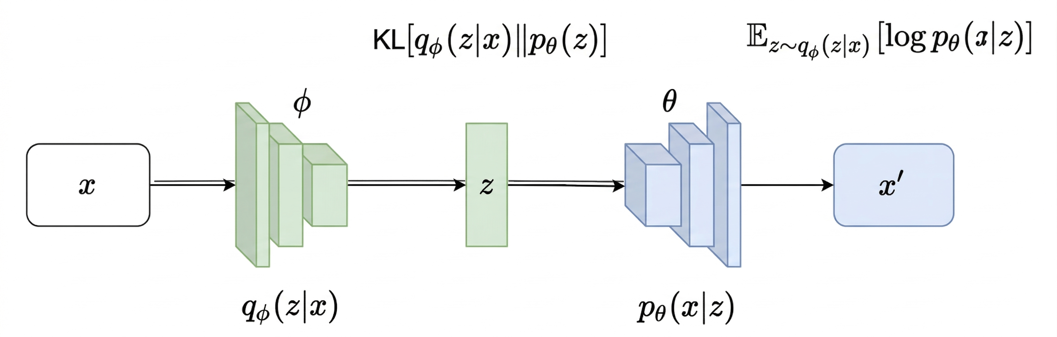
A VAE: encoder $q_\phi(z\mid x)$ approximating the posterior, decoder $p_\theta(x\mid z)$.
A VAE learns a joint $p_\theta(x,z)$ via an encoder $q_\phi(z\mid x)$ and decoder
$p_\theta(x\mid z)$, maximizing the evidence lower bound
$$ \c{L}_{\mathrm{ELBO}}(x;\theta,\phi)=\underbrace{\EE_{q_\phi(z\mid x)}[\log p_\theta(x\mid z)]}_{\text{reconstruction}}-\underbrace{\mathrm{KL}\!\smbr{q_\phi(z\mid x)\,\|\,p(z)}}_{\text{regularization}}. $$
Variational continual learning (VCL) reframes stability–plasticity as sequential
Bayesian updating. At stage $t$ with data $x_t$,
$$ \c{L}_t(\theta,\phi;x_t)=\EE_{z\sim q_\phi(z\mid x_t)}[\log p_\theta(x_t\mid z)]-\mathrm{KL}\!\sqbr{q_\phi(z\mid x_t)\,\|\,p_{\mathrm{prior}}(z)}, $$
with two strategies.2 The likelihood-focused strategy (generative
replay) hallucinates data from stages $
§3. Generative replay for diffusion
Continually train a diffusion model across tasks $t=1,\dots,T_{\mathrm{tasks}}$ without storing past real data.3 With $\theta_{t-1}$ the frozen previous noise predictor, $r\in(0,1)$ a task-importance ratio, and the standard loss $\c{L}_{\mathrm{simple}}(x;\theta)=\EE_{\tau,\epsilon}\sqbr{\norm{\epsilon-\epsilon_\theta(x_\tau,\tau)}_2^2}$, task 1 trains $\theta_1$ on real $X_1$. For $t>1$: generate replay $X_{\mathrm{replay}}=\mathrm{DDIM}(x_T;\theta_{t-1})$ from noise $x_T\sim\c{N}(0,I)$, then minimize the mixed objective $$ \c{L}_{\mathrm{GR}}(\theta_t)=r\,\EE_{x\sim X_t}[\c{L}_{\mathrm{simple}}(x;\theta_t)]+(1-r)\,\EE_{\hat x\sim X_{\mathrm{replay}}}[\c{L}_{\mathrm{simple}}(\hat x;\theta_t)]. $$ Because the diffusion model itself is the target (no separate solver), replay data simply enters the same denoising loss — the diffusion form of the generative-replay term.
§4. Why DDIM is deterministic
Standard DDPM uses a Markovian reverse process injecting fresh noise at every step. DDIM generalizes to a non-Markovian process with a variance parameter $\sigma_\tau$: $$ x_{\tau-1}=\sqrt{\alpha_{\tau-1}}\underbrace{\smbr{\frac{x_\tau-\sqrt{1-\alpha_\tau}\,\epsilon_\theta(x_\tau,\tau)}{\sqrt{\alpha_\tau}}}}_{\text{predicted }x_0}+\underbrace{\sqrt{1-\alpha_{\tau-1}-\sigma_\tau^2}\,\epsilon_\theta(x_\tau,\tau)}_{\text{direction to }x_\tau}+\underbrace{\sigma_\tau\epsilon}_{\text{noise}}. $$
Setting $\sigma_\tau=0$ for all $\tau$ kills the noise term; the generation collapses into an
Euler step of the underlying probability-flow ODE. Consequence for replay:
once the latent $x_T\sim\c{N}(0,I)$ is fixed, the whole trajectory
$x_T\to\dots\to x_0$ is completely determined by $\theta_{t-1}$ — so the synthetic replay set
is reproducible, not a fresh random draw each time.
1 Prabhu et al., “GDumb,” ECCV 2020; Lopez-Paz & Ranzato (GEM), NeurIPS 2017. 2 Nguyen et al., “Variational continual learning,” arXiv:1710.10628. 3 Masip et al., “Continual learning of diffusion models with generative distillation,” arXiv:2311.14028; Ho, Jain & Abbeel, arXiv:2006.11239. — the classical-foundations talk is March 19; the full algorithm taxonomy is algorithms for CL with diffusion.
Talk — continual learning: classical foundations
Slide notes from a talk walking the classical half of these notes end to end: from the foundational distinction and desiderata, through McCloskey's experiment and the three scenarios, the performance matrix, and the two regularization methods that anchor the field. Most of the material has its own entry; I record the roadmap here and write out the one piece the survey did not yet cover — Learning without Forgetting, and how it contrasts with EWC.
Roadmap
- Foundational distinction and desiderata → formalisms and desiderata
- Short history; McCloskey's A–B / A–C experiment → McCloskey–Cohen
- The modern diffusion-model analogue → problem statements
- Classical formalism; three scenarios; Split MNIST → definitions of tasks
- Performance matrix; ACC/BWT/FM/FWT; vector-valued generative metrics → §3, metrics
- Three mitigation strategies; EWC and its Fisher; worked example → forgetting and EWC
- Learning without Forgetting; EWC vs. LwF → below
§1. Learning without Forgetting (LwF)
Setting: a pretrained network with shared parameters $\theta_s$ and old-task parameters $\theta_o$; a new task arrives with data $(X_n,Y_n)$, but the old training data are unavailable.1 The construction:
- Record the old model's responses on the new-task inputs, $Y_o\leftarrow\mathrm{CNN}(X_n;\theta_s,\theta_o)$.
- Add new task-specific parameters $\theta_n$.
- Train by minimizing $$ \min_{\hat\theta_s,\hat\theta_o,\hat\theta_n}\sqbr{\lambda_o\,L_{\mathrm{old}}(Y_o,\hat Y_o)+L_{\mathrm{new}}(Y_n,\hat Y_n)+R(\hat\theta_s,\hat\theta_o,\hat\theta_n)}, $$ where $L_{\mathrm{new}}$ fits the new labels and $L_{\mathrm{old}}$ keeps the old outputs close on the same inputs.
So LwF is fine-tuning with an output-preservation constraint — it needs no old data, only the old model's predictions on the new inputs.
§2. EWC vs. LwF: two notions of stability
EWC protects parameters locally important for the old task —
$\theta\approx\theta_A^\ast$ in high-Fisher directions — so the old task is preserved in
weight space.
LwF preserves the old model's responses on new-task inputs, $\hat Y_o\approx Y_o$, so the old task is preserved in prediction space.
LwF preserves the old model's responses on new-task inputs, $\hat Y_o\approx Y_o$, so the old task is preserved in prediction space.
The conceptual contrast: EWC asks which parameters should not move?; LwF asks which outputs should remain stable? That weight-space vs. function-space split is exactly the axis the diffusion methods inherit in function-space consolidation (e.g. matching diffusion classifier scores) versus Fisher penalties.
1 Li & Hoiem, “Learning without forgetting,” ECCV 2016; Kirkpatrick et al., “Overcoming catastrophic forgetting,” PNAS 2017. — the companion talk on replay and diffusion is March 26.
The closed immersion $[X/B]\hookrightarrow [Y/B]$ and its pushforward
Packages the computation of S4 into a morphism of quotient stacks and identifies the resulting $K$-theory class as the SL$_2$/$s_\alpha$ piece of Antor's convolution basis. Depends on foundation F3 for quotient stacks and closed immersions.
§1. The closed immersion
From S4 §5, $X = V(y,p,xq)$ is a $B$-stable closed subscheme of $Y = Y_{SL_2} = V(py,\ px-qy,\ qx)$. By F3 §3, the induced morphism of quotient stacks $$ i : [X/B] \;\hookrightarrow\; [Y/B] $$ is a closed immersion.
§2. Derived pushforward of the structure sheaf
Closed immersions have exact pushforward, so $$ R i_* \mathcal O_{[X/B]} \;\cong\; i_* \mathcal O_{[X/B]}, $$ concentrated in homological degree $0$. Via the equivalence $\operatorname{QCoh}([Y/B]) \simeq \operatorname{QCoh}^B(Y)$ (F3 §2), this pushforward corresponds to the $B$-equivariant $\mathcal O_Y$-module $$ i_* \mathcal O_{[X/B]} \;\cong\; \mathcal O_Y\,/\,(y,\ p). $$ Here the ideal $(y,p)$ is understood in $\mathcal O_Y = \mathbf{C}[x,y,p,q]/(py,\ px-qy,\ qx)$; the equations $py, px-qy$ become trivial after imposing $y=p=0$, and $qx$ survives to cut out the component structure of $X$.
§3. Identification with Antor's convolution basis
Antor's theorem gives the $K$-theoretic realization $$ K^{G\times \mathbb G_m^I}(Z) \;\cong\; \mathcal H^{\mathrm{aff}}_{\mathbf q} $$ of the affine Hecke algebra with (unequal) parameters, where $Z = \tilde V\times_V\tilde V$ is the associated Steinberg-type variety. The isomorphism carries the basis $\{[\mathcal O_{\overline{Z_w}}]\}_{w\in W}$, indexed by the Weyl group, to the canonical $K$-theoretic basis on the Hecke side. See Ant25, Lem. 2.5 (p. 8–9), Prop. 2.16 (p. 12), Thm. A (p. 3).
In the SL$_2$/$s_\alpha$ case, $W = \{\mathrm{id}, s_\alpha\}$. The class $[\mathcal O_{\overline{Z_{\mathrm{id}}}}]$ corresponds to the identity diagonal $Z_\Delta\subset Z$; the class $[\mathcal O_{\overline{Z_{s_\alpha}}}]$ is exactly the class computed above, namely $$ [\mathcal O_{[X/B]}] \;=\; [\mathcal O_Y/(y,p)] \;\in\; K^B(Y) \;\cong\; K^{B\times\mathbb G_m^I}(Z) $$ after transporting along the usual identification of $Y_{SL_2}$ with its Springer/Steinberg counterpart.
§4. Remark on the $Y_B$-ambient version
If one works with $[X/B]\hookrightarrow[Y_B/B]$ instead of $[Y/B]=[Y_{SL_2}/B]$, then (S4 §6) $X$ is replaced by $\overline{T^*_O V} = V(y,p)$ itself, and the pushforward simplifies to $\mathcal O_{Y_B}/(y,p) = \mathcal O_{V(y,p)}$ as a $B$-equivariant sheaf. The convolution-basis interpretation is cleaner there, at the cost of enlarging the ambient scheme.
§5. $X\hookrightarrow Y$ as a toy relative correspondence
Antor's $Z = \widetilde V\times_V \widetilde V$ is a self-fiber product: two copies of the Springer-type space $\widetilde V$ glued over $V$. In [LPY25], the analogous object at the Iwahori level of the local relative Langlands conjecture is the relative Steinberg kernel $$ \widetilde{\check{\mathfrak g}}^{,*}(2)\ \times_{\check{\mathfrak g}^{*}(2)}\ \check M, $$ where one Grothendieck–Springer leg is kept and the other is replaced by the dual Hamiltonian space $\check M$ of a spherical $G$-variety $X$ (Thm. 1.3 / Thm. 5.1). See F4 for the comparison in detail.
Our $[X/B]\hookrightarrow[Y/B]$ is not a self-fiber product: we embed a single distinguished closed subscheme (the conormal-closure leg) into the ambient moment-zero fiber $Y$, and in that sense it is a local coordinate-level model of the asymmetric “one leg fixed, the other leg replaced by a $G$-Hamiltonian object” architecture that appears in [LPY25]. The derived refinement of our scheme-theoretic intersection is $\overline{T^*_O V}\cap^R_{T^*V} Y$, whose $\mathcal O$-algebra is $\mathcal O_{\overline{T^*_O V}}\otimes_{\mathcal O_{T^*V}}^L \mathcal O_Y$; by BFN this corresponds to the relative tensor product $\mathrm{Perf}(\overline{T^*_O V})\otimes_{\mathrm{Perf}(T^*V)}\mathrm{Perf}(Y)$.
So the full conceptual chain reads: convolution-basis element $[\mathcal O_{[X/B]}]$ $\to$ local relative correspondence $X\hookrightarrow Y$ $\to$ derived intersection $\overline{T^*_O V}\cap^R Y$ $\to$ relative tensor product of categories $\to$ categorified relative Hecke/Satake action of [LPY25].
cf. Ant25, Lem. 2.5 (p. 8–9) on $K^H(Z)$ as a free $K^H(Z_\Delta)$-module with basis $\{[\mathcal O_{\overline{Z_w}}]\mid w\in W\}$; Prop. 2.16 (p. 12) for the convolution formula; Thm. A / Thm. 2.19 (p. 3) for the main isomorphism. LPY25 = Lin–Pham–Yu, arXiv:2510.25231, Thm. 1.3 (p. 3) for the relative Steinberg kernel; Ben-Zvi–Francis–Nadler, Integral transforms and Drinfeld centers in derived algebraic geometry, for $\mathrm{QCoh}(X\times_S^R Y)\simeq \mathrm{QCoh}(X)\otimes_{\mathrm{QCoh}(S)}\mathrm{QCoh}(Y)$.
The $SL_2$-moment map and the zero fibers $Y_{SL_2}$, $Y_B$
Explicit computation of the cotangent-lift moment map for $SL_2 \curvearrowright T^*V$ on $V = \mathbf{A}^2$. Depends on S1 (conventions and cotangent lift) and F1 (cotangent-lift formula). Output: two ideals $Y_{SL_2}$ and $Y_B$ that are the ambient zero fibers used downstream.
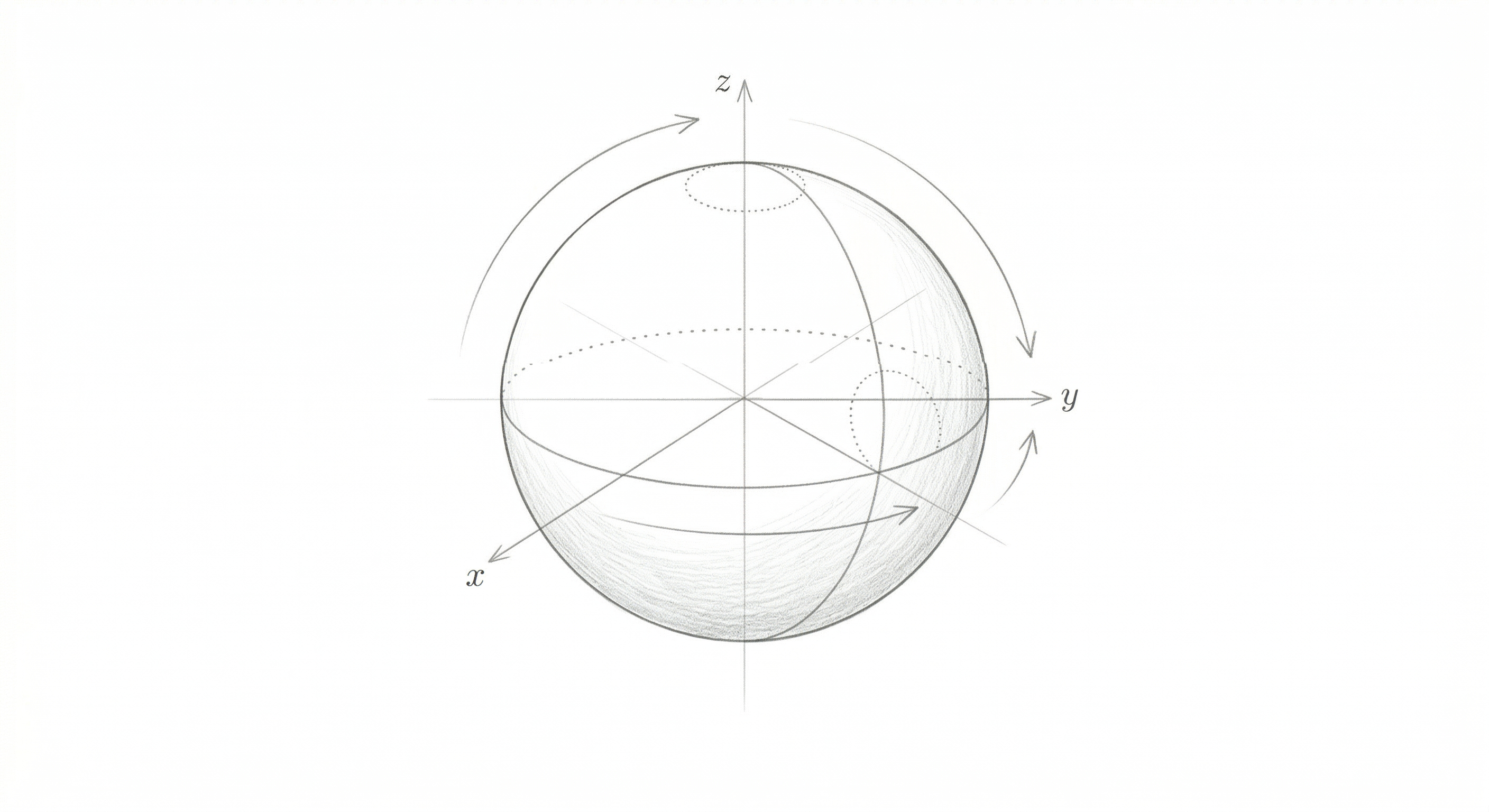
§1. Fundamental vector fields
Use the standard basis of $\mathfrak{sl}_2$: $$ e \;=\; \begin{pmatrix}0&1\\0&0\end{pmatrix}, \qquad h \;=\; \begin{pmatrix}1&0\\0&-1\end{pmatrix}, \qquad f \;=\; \begin{pmatrix}0&0\\1&0\end{pmatrix}, $$ and the convention $\xi_V(v) = \tfrac{d}{dt}|_{t=0}\exp(t\xi)\cdot v$ fixed in F1 §5. For the defining action $\xi\cdot(x,y) = \xi\bigl[\begin{smallmatrix}x\\y\end{smallmatrix}\bigr]$ we compute: $$ e \cdot \begin{pmatrix}x\\y\end{pmatrix} = \begin{pmatrix}y\\0\end{pmatrix}, \qquad h \cdot \begin{pmatrix}x\\y\end{pmatrix} = \begin{pmatrix}x\\-y\end{pmatrix}, \qquad f \cdot \begin{pmatrix}x\\y\end{pmatrix} = \begin{pmatrix}0\\x\end{pmatrix}. $$ As vector fields on $V$: $$ e_V \;=\; y\,\partial_x,\qquad h_V \;=\; x\,\partial_x \;-\; y\,\partial_y,\qquad f_V \;=\; x\,\partial_y. $$
§2. The $SL_2$-moment map
Pairing with $\alpha = p\,dx + q\,dy$ via the cotangent-lift formula $\langle \mu(v,\alpha),\xi\rangle = \alpha(\xi_V(v))$ (F1 §3): $$ \langle \mu_{SL_2},\,e\rangle \;=\; py, \qquad \langle \mu_{SL_2},\,h\rangle \;=\; px - qy, \qquad \langle \mu_{SL_2},\,f\rangle \;=\; qx. $$ Using the dual basis $\{e^*,h^*,f^*\}$ to write $\mathfrak{sl}_2^*$-coordinates, $$ \mu_{SL_2}(x,y,p,q) \;=\; (py,\ px - qy,\ qx). $$ The sign is fixed by our convention (F1 §5); the zero fiber is independent of the sign.
Equivalently, in the $\mathrm{GL}(V)$ form (F1 §4): $\mu_{\mathrm{GL}(V)}(v,\alpha) = v\otimes\alpha = \bigl[\begin{smallmatrix} px & py \\ qx & qy \end{smallmatrix}\bigr]$, and restricting to $\mathfrak{sl}_2 \subset \mathfrak{gl}_2$ means pairing with traceless matrices; the three components above are the pairings with $e$, $h/2$ (up to scale), and $f$ respectively.
§3. The zero fiber $Y_{SL_2} := \mu_{SL_2}^{-1}(0)$
$$ Y_{SL_2} \;=\; \operatorname{Spec} \mathbf{C}[x,y,p,q]\,/\,(py,\ px - qy,\ qx). $$ This is a three-dimensional reducible affine variety in $T^*V = \mathbf{A}^4$. Geometrically it is the union of conormals to the two $SL_2$-orbits on $V$ (namely $V\setminus\{0\}$ and $\{0\}$); cf. F2 §2 and S3.
§4. The $B$-moment map and $Y_B$
The Borel Lie algebra is $\mathfrak b = \langle e,h\rangle \subset \mathfrak{sl}_2$, so by F1 §2 the $B$-moment map is the projection $$ \mu_B \;=\; \mu_{SL_2}\big|_{\mathfrak b} \;=\; (py,\ px - qy). $$ Its zero fiber is $$ Y_B \;=\; \operatorname{Spec}\mathbf{C}[x,y,p,q]\,/\,(py,\ px - qy), $$ strictly larger than $Y_{SL_2}$: the relation $qx=0$ is dropped. Concretely, $Y_B \supsetneq Y_{SL_2}$, with the difference accounted for by points where $p$ vanishes and the remaining equations force no constraint on $qx$.
§5. Dictionary with Antor
Neither $Y_{SL_2}$ nor $Y_B$ is the Steinberg-type variety $Z = \tilde V\times_V \tilde V$ of Antor; they live in $T^*V = V\times V^*$, whereas $Z$ lives in $\tilde V\times\tilde V$. The match is only set up after the identification of $T^*\mathcal B$ with a Springer-type bundle and the reduction by the moment map; see Ant25, p. 7. For this note, the relevant fact is that the pieces of $Y_{SL_2}$ we need in S3–S4 are the SL$_2$-analogues of $\overline{Z_w}$.
cf. Ant25, p. 7 for $\tilde V$, $\mu:\tilde V\to V$, and $Z := \tilde V\times_V \tilde V$.
$B$-orbits on $\mathbf{A}^2$ and their conormal bundles
Classifies the three $B$-orbits on $V = \mathbf{A}^2$, computes each conormal bundle $T^*_O V \subset T^*V$, and identifies $\mu_B^{-1}(0)$ set-theoretically as their union. Depends on S1 (the $B$-action), S2 (the moment map), and foundation F2 (conormal vs cotangent).
§1. The three $B$-orbits
Under the standard left $B$-action on $V$ there are exactly three orbits: $$ O_{\mathrm{open}} \;=\; \{(x,y): y\neq 0\}, \quad O_x \;=\; \{(x,0): x\neq 0\}, \quad O_0 \;=\; \{(0,0)\}. $$
Proof. If $y\neq 0$, choose $a = y$ and $b = -x$; then $$ \begin{pmatrix} a & b \\ 0 & a^{-1}\end{pmatrix}\cdot (x,y) \;=\; (ax + by,\ a^{-1}y) \;=\; (xy - xy,\ 1) \;=\; (0,1), $$ so every $(x,y)$ with $y\neq 0$ lies in the orbit of $(0,1)$. If $y = 0$ and $x\neq 0$, choose $a = x^{-1}$ and $b = 0$: $(x,0)\mapsto (1,0)$, so the $\{y=0,\ x\neq 0\}$-slice is a single orbit. The origin is $B$-fixed because both coordinates are homogeneous. Hence three orbits.
Closure relations. $\overline{O_{\mathrm{open}}} = V$, $\overline{O_x} = \{y=0\}$, $\overline{O_0} = \{(0,0)\}$. Thus $O_0 \subset \overline{O_x} \subset \overline{O_{\mathrm{open}}}$.
§2. Conormal bundles of the three orbits
Recall (F2 §1) that $(T^*_O V)_x = \{\alpha\in T^*_xV : \alpha|_{T_xO}=0\}$.
- $O_{\mathrm{open}}$ is open in $V$, so $T_xO_{\mathrm{open}} = T_xV$ for every $x\in O_{\mathrm{open}}$. The conormal fiber is zero, so $$ T^*_{O_{\mathrm{open}}}V \;=\; \{(x,y,0,0):y\neq 0\} \;\subset\; T^*V. $$ Its closure in $T^*V$ is the zero section, $\{(x,y,0,0)\} = V(p,q)$.
- $O_x = \{(x,0):x\neq 0\}$. The tangent line at $(x,0)$ is $T_{(x,0)}O_x = \langle\partial_x\rangle$; a covector $p\,dx+q\,dy$ annihilates $\partial_x$ iff $p=0$. So $$ T^*_{O_x}V \;=\; \{(x,0,0,q): x\neq 0\}. $$ Taking closures in $T^*V$: $$ \overline{T^*_{O_x}V} \;=\; V(y,\,p) \;=\; \{(x,0,0,q)\} \;\subset\; T^*V. $$ This is the two-dimensional variety that will play the starring role in S4.
- $O_0 = \{(0,0)\}$. The tangent space is zero, so the conormal fiber is the whole cotangent fiber: $$ T^*_{O_0}V \;=\; \{(0,0,p,q)\} \;=\; V(x,y) \;\subset\; T^*V. $$ Already closed.
§3. Union-of-conormals interpretation of the zero fibers
By foundation F2 §2, $\mu_B^{-1}(0)$ is set-theoretically the union of conormals to the $B$-orbits. Writing these in the closures we have just computed: $$ \mu_B^{-1}(0) \;=\; \overline{T^*_{O_{\mathrm{open}}}V}\ \cup\ \overline{T^*_{O_x}V}\ \cup\ T^*_{O_0}V \;=\; V(p,q)\ \cup\ V(y,p)\ \cup\ V(x,y). $$ Check that this is consistent with $Y_B = V(py,\ px-qy)$ from S2 §4. A point $(x,y,p,q)$ lies in $Y_B$ iff $py=0$ and $px=qy$.
- If $p=0$ and $q=0$, both equations hold; this is the zero section $V(p,q) = \overline{T^*_{O_{\mathrm{open}}}V}$.
- If $p=0,\ y=0$, then $py=0$ automatically and $px=qy$ becomes $0=0$, again automatic. So the two-plane $V(y,p)=\overline{T^*_{O_x}V}$ lies in $Y_B$.
- If $x=0,\ y=0$, again both equations are trivially satisfied; the fiber $V(x,y) = T^*_{O_0}V$ lies in $Y_B$.
Conversely, any $(x,y,p,q)\in Y_B$ with $(y,p)\neq (0,0)$ must have $y=0\Rightarrow p=0$ or $p=0$ (from $py=0$); the second equation then forces further constraints landing the point in one of the three sets above. Set-theoretic equality.
For $\mu_{SL_2}^{-1}(0) = V(py,\ px-qy,\ qx)$ the analogous statement uses the two $SL_2$-orbits on $V$: $V\setminus\{0\}$ and $\{0\}$. Their conormal bundles are $V(p,q)$ (zero section over $V\setminus\{0\}$, closure adds the cotangent fiber at the origin to give $V(p,q)$) and $V(x,y)$. So $$ \mu_{SL_2}^{-1}(0) \;=\; V(p,q)\ \cup\ V(x,y) \qquad (\text{set-theoretically}). $$
§4. The specific orbit we care about
The main argument works with $O := O_x = B\cdot(1,0)$. Its conormal closure $\overline{T^*_O V} = V(y,p)$ is a $B$-stable two-dimensional subvariety of $T^*V$. It is not equal to $V(y,p,xq)$. The scheme $V(y,p,xq)$ appears only after intersecting $\overline{T^*_O V}$ with $Y_{SL_2}$; that intersection is the subject of S4, which also supersedes the corresponding claim in the old monolithic note.
cf. Ant25, Lem. 2.14 (p. 11) on the $P_\alpha$-stability of $V^-\cap{}^{s_\alpha}V^-$, which in the SL$_2$ case is the line $\operatorname{span}\{y\}$.
The $B$-action on $\mathbf{A}^2$ and its cotangent lift
Fixes the conventions for the rest of the SL$_2$/$B$ note: coordinates on $V$ and on $T^*V$, the standard left $B$-action on $V$, and the canonically lifted $B$-action on $T^*V$. Foundation F3 covers left/right conventions and the associated bundle $G\times^B V^-$.
§1. Coordinates
Let $V = \mathbf{A}^2 = \operatorname{Spec}\mathbf{C}[x,y]$ with coordinates $(x,y)$, and identify $$ T^*V \;=\; \operatorname{Spec}\mathbf{C}[x,y,p,q], $$ where $p,q$ are the coordinates dual to $x,y$, so a cotangent covector at $(x,y)$ is written $\alpha = p\,dx + q\,dy$.
Let $G = SL_2(\mathbf{C})$ and let $$ B \;=\; \left\{\begin{pmatrix} a & b \\ 0 & a^{-1} \end{pmatrix} : a \in \mathbf{C}^\times,\ b\in \mathbf{C}\right\} \;\subset\; G $$ be the upper-triangular Borel.
§2. The left $B$-action on $V$
Take the standard left action of $B$ on $V$: $$ \begin{pmatrix} a & b \\ 0 & a^{-1} \end{pmatrix} \cdot (x,y) \;=\; (ax + by,\ a^{-1} y). $$ Check of the action axioms: matrix multiplication $\bigl[\begin{smallmatrix} a_1&b_1\\0&a_1^{-1}\end{smallmatrix}\bigr] \bigl[\begin{smallmatrix} a_2&b_2\\0&a_2^{-1}\end{smallmatrix}\bigr] = \bigl[\begin{smallmatrix} a_1a_2 & a_1b_2+b_1a_2^{-1}\\0&(a_1a_2)^{-1}\end{smallmatrix}\bigr]$, and applying this to $(x,y)$ gives $(a_1a_2\,x + (a_1b_2+b_1a_2^{-1})y,\ (a_1a_2)^{-1}y)$, which matches the composite $\bigl[\begin{smallmatrix} a_1&b_1\\0&a_1^{-1}\end{smallmatrix}\bigr]\cdot \bigl(\bigl[\begin{smallmatrix} a_2&b_2\\0&a_2^{-1}\end{smallmatrix}\bigr]\cdot(x,y)\bigr)$. Identity acts trivially.
As a $B$-module $V$ has weights under the torus $T = \{\operatorname{diag}(a,a^{-1})\}$: the vector $y$ has weight $-\alpha$ (where $\alpha$ is the positive simple root, $\operatorname{diag}(a,a^{-1})\mapsto a^2$), and $x$ has weight $+\alpha$. The unipotent part $U = \{b\mapsto[\begin{smallmatrix}1&b\\0&1\end{smallmatrix}]\}$ sends $y$ to $by+(\text{lower weights})$; concretely $[\begin{smallmatrix}1&b\\0&1\end{smallmatrix}]\cdot (x,y) = (x+by,\ y)$, so $y$ is $U$-invariant and $x$ is not.
§3. Cotangent lift
Cotangent lifts are characterized by: $(g,(x,\alpha))\mapsto (g\cdot x,\ (g^*)^{-1}\alpha)$ where $g^*$ is the pullback along the action by $g$. Concretely, write the $B$-action on $V$ as the linear map $$ L_{(a,b)} = \begin{pmatrix} a & b \\ 0 & a^{-1}\end{pmatrix}. $$ Then $(L_{(a,b)}^*)^{-1} = (L_{(a,b)}^{-1})^*$, and $L_{(a,b)}^{-1} = \bigl[\begin{smallmatrix} a^{-1} & -b \\ 0 & a\end{smallmatrix}\bigr]$. Its transpose sends the dual basis $(dx, dy)$ to $$ (dx, dy)\ \longmapsto\ (a^{-1}\,dx,\ -b\,dx + a\,dy). $$ So the cotangent components $(p,q)$ transform as the inverse-transpose of the tangent components, yielding $$ \begin{pmatrix} a & b \\ 0 & a^{-1} \end{pmatrix}\cdot (x,y,p,q) \;=\; (ax + by,\ a^{-1}y,\ a^{-1}p,\ -bp + aq). $$
Sanity check. Evaluate on the pure torus part $b=0$: $(x,y,p,q)\mapsto(ax,a^{-1}y,a^{-1}p,aq)$, which is the correct contragredient behavior on cotangent coordinates. Evaluate on pure unipotent $a=1$: $(x,y,p,q)\mapsto(x+by,y,p,-bp+q)$; check $\omega = dp\wedge dx + dq\wedge dy$ is preserved: $d(p)\wedge d(x+by) + d(-bp+q)\wedge dy = dp\wedge dx + b\,dp\wedge dy - b\,dp\wedge dy + dq\wedge dy = dp\wedge dx + dq\wedge dy = \omega$. OK.
§4. $V^-$ for the associated bundle $\tilde V$
Antor's framework needs a $B$-stable subspace $V^- \subset V$ to form $\tilde V = G \times^B V^-$. In the SL$_2$/$\mathbf{A}^2$ case the unique non-trivial choice is $$ V^- \;=\; \operatorname{span}\{y\}, $$ the $(-\alpha)$-weight line. It is $B$-stable because $B$ acts on $y$ by the character $\chi(a,b) = a^{-1}$, i.e. $[\begin{smallmatrix}a&b\\0&a^{-1}\end{smallmatrix}]\cdot y = a^{-1}y$. The image of the zero section of $\tilde V = G\times^B V^- \to \mathcal B$ is the $B$-orbit closure $\{y = 0\}\subset V$. See Ant25, Def. 2.13 and Lem. 2.14 (p. 11).
cf. Ant25, §2.1 (p. 6) on $B$-modules $W$ and the induced $G$-equivariant bundle $\pi : G\times^B W \to \mathcal B$; Def. 2.13 (p. 11) for the rooted representation condition.
The subscheme $X = V(y,p,xq)$ as an intersection, not a conormal closure
Defines the closed subscheme $X \subset T^*V$ that carries the main argument and corrects the conflation between “conormal closure” and “conormal closure intersected with the moment-zero fiber.” Depends on S2 (for $Y_{SL_2}$, $Y_B$), S3 (for $\overline{T^*_O V} = V(y,p)$), and foundation F2.
Correction. $X$ is not itself the conormal bundle closure. The
conormal closure of $O = B\cdot(1,0)$ is $\overline{T^*_O V} = V(y,p)$, a two-dimensional
subvariety of $T^*V$. The subscheme $X = V(y,p,xq)$ is strictly smaller: it is
$\overline{T^*_O V}$ intersected with $Y_{SL_2}$. This distinction matters because
$\overline{T^*_O V}$ is smooth and irreducible away from the zero section, while $X$ is
one-dimensional with two components. The old monolithic note §5 was ambiguous on this;
this page is the clean version.
§1. Definition of $X$
Set $O := B\cdot(1,0) = \{(x,0):x\neq 0\}$. Using $\overline{T^*_O V} = V(y,p)$ from S3 and $Y_{SL_2} = V(py,\ px-qy,\ qx)$ from S2, define $$ X \;:=\; \overline{T^*_O V}\ \cap\ Y_{SL_2} \;\subset\; T^*V. $$
§2. Computation: $X = V(y,p,xq)$
Impose $y=0$ and $p=0$ in the three generators of the $Y_{SL_2}$ ideal: $$ py\big|_{y=0,p=0} = 0, \qquad px - qy\big|_{y=0,p=0} = 0, \qquad qx\big|_{y=0,p=0} = qx. $$ Two of the three relations become trivial; only $qx = 0$ survives. Hence $$ X \;=\; \operatorname{Spec}\mathbf{C}[x,y,p,q]\,/\,(y,\ p,\ xq). $$ Because the ideal is generated by a regular sequence—well, almost: $(y,p)$ is regular, and $xq$ is a zero-divisor modulo $(y,p)$—the intersection is not transverse at the origin; see §4.
§3. Reduced structure and irreducible components
The ideal $(y,\ p,\ xq) \subset \mathbf{C}[x,y,p,q]$ decomposes as $$ (y,\ p,\ xq) \;=\; (y,\ p,\ x)\ \cap\ (y,\ p,\ q). $$ So $X$ has exactly two irreducible components, each one-dimensional: $$ X_1 \;=\; V(y,p,q) \;=\; \{(x,0,0,0)\} \quad \text{(the $x$-axis)}, $$ $$ X_2 \;=\; V(y,p,x) \;=\; \{(0,0,0,q)\} \quad \text{(the $q$-axis)}, $$ meeting transversally at the origin. Component $X_1$ is the closure in $T^*V$ of the orbit $O$ viewed as the zero section above it; component $X_2$ is the covector fiber at the origin constrained by $p=0$.
§4. Why $X\neq \overline{T^*_O V}$
$\overline{T^*_O V} = V(y,p)$ is the two-plane $\{(x,0,0,q)\}$, which is two-dimensional. $X = V(y,p,xq)$ is a one-dimensional subscheme sitting inside this two-plane and is carved out by the extra equation $xq=0$. Concretely, $$ \overline{T^*_O V}\ \setminus\ X \;=\; \{(x,0,0,q):x\neq 0,\ q\neq 0\}, $$ which is a two-dimensional open subset of the two-plane. The extra equation $xq=0$ comes from the residual $f$-component $qx$ of $\mu_{SL_2}$; the $B$-moment map has no such component, so this reduction only happens when we work with $Y_{SL_2}$ rather than $Y_B$.
§5. $B$-stability
$X$ is $B$-stable because both $\overline{T^*_O V}$ and $Y_{SL_2}$ are $B$-stable:
- $Y_{SL_2}$ is $SL_2$-stable (hence $B$-stable) since the moment map is $SL_2$-equivariant.
- $\overline{T^*_O V}$ is $B$-stable because the conormal bundle of a $B$-orbit is $B$-invariant, and the closure of a $B$-invariant set is $B$-invariant.
Explicitly, using the cotangent lift formula from S1 §3, if $y=0$ and $p=0$ then $\bigl[\begin{smallmatrix}a&b\\0&a^{-1}\end{smallmatrix}\bigr]\cdot(x,0,0,q)=(ax,0,0,aq)$, which preserves both $y=0$ and $p=0$, and sends $xq\mapsto (ax)(aq)=a^2 xq$, preserving $xq=0$.
§6. The $B$-moment variant
If instead one ambient-moment-zero fiber is $Y_B = V(py,\ px-qy)$ rather than $Y_{SL_2}$, then $\overline{T^*_O V} = V(y,p)$ already lies entirely inside $Y_B$: both relations $py$ and $px-qy$ vanish after setting $y=0$ and $p=0$. So $$ \overline{T^*_O V}\ \cap\ Y_B \;=\; \overline{T^*_O V} \;=\; V(y,p). $$ No intersection step is needed. In that version conormal closures appear as intrinsic closed subvarieties of $Y_B$, not as residual intersections. This is the cleaner presentation for the $B$-side; the $Y_{SL_2}$-version (the main argument) carries the extra $xq=0$ constraint.
cf. Ant25, Lem. 2.15 (p. 12): $\Lambda_{s_\alpha} = \overline{Z_{s_\alpha}}$; Lem. 2.4 (p. 8): $Z_w \to Y_w$ is a $G$-equivariant vector bundle. Derived-intersection interpretation: the scheme-theoretic $X = \overline{T^*_O V}\cap Y_{SL_2}$ is the $t_0$-truncation of the derived intersection $\overline{T^*_O V}\cap^R_{T^*V} Y_{SL_2}$, with $\mathcal O^L \simeq \mathcal O_{\overline{T^*_O V}}\otimes_{\mathcal O_{T^*V}}^L\mathcal O_{Y_{SL_2}}$; by Ben-Zvi–Francis–Nadler (BFN10) the corresponding category of perfect complexes is the relative tensor product $\mathrm{Perf}(\overline{T^*_O V})\otimes_{\mathrm{Perf}(T^*V)}\mathrm{Perf}(Y_{SL_2})$. This is the “derived” version of the one-leg-fixed architecture used at the categorical level in LPY25, §1 (Thm. 1.3); see also F4.
Relative Langlands motivation: from Antor's self-Steinberg to the LPY relative Steinberg
Why should one care about an SL$_2$-toy of the intersection $X = \overline{T^*_O V}\cap Y$? Because the step from Chriss–Ginzburg / Antor to the tamely ramified local relative Langlands picture is exactly the step from a self-fiber product (Steinberg) to a one-sided relative fiber product, and our $X\hookrightarrow Y$ is a local coordinate-level model of that passage. The reference for the relative case is [LPY25].
§1. Classical Steinberg (Chriss–Ginzburg / Kazhdan–Lusztig)
For a connected reductive group $G$, the Steinberg variety is the self-fiber product $$ \mathrm{St} \;=\; \widetilde{\mathfrak g}\times_{\mathfrak g}\widetilde{\mathfrak g} \qquad\bigl(\text{or}\quad \widetilde{\mathcal N}\times_{\mathcal N}\widetilde{\mathcal N}\bigr), $$ where $\widetilde{\mathfrak g}\to\mathfrak g$ is the Grothendieck–Springer resolution. Convolution on $K$-theory realizes the affine Hecke algebra. The geometric input is a self-correspondence over the Lie-theoretic base; the algebraic output is an algebra.
§2. Antor: self-Steinberg for a rooted representation
[Ant25] keeps the self-correspondence architecture but replaces $\mathfrak g$ by a rooted $G$-representation $V$. Setting $\widetilde V = G\times^B V^-\to V$, the geometric object is again a self-fiber product $$ Z \;=\; \widetilde V\times_V \widetilde V, $$ and convolution on $K^{G\times\mathbb G_m^I}(Z)$ realizes the affine Hecke algebra $\mathcal H^{\mathrm{aff}}_{\mathbf q}$ with unequal parameters (Ant25, Thm. A (p. 3), Prop. 2.16 (p. 12)). Antor explicitly notes the scheme-theoretic vs reduced fiber product makes no difference at the level of $K$-theory.
§3. LPY: the relative Steinberg kernel
[LPY25] works at the categorical level and makes the problem relative. Fix a smooth affine spherical $G$-variety $X$ satisfying the unramified local relative Langlands equivalence and Ras's dimension theory (Assumption 1.2, p. 3). The spectral kernel for the Iwahori-level Satake subcategory is $$ \widetilde{\check{\mathfrak g}}^{,*}(2)\times_{\check{\mathfrak g}^{*}(2)} \check M \;\subset\; \widetilde{\check{\mathfrak g}}^{,*}(2)\;\times\;\check M, $$ where $\widetilde{\check{\mathfrak g}}^*(2) = T^*(2)(\check G/\check N)/\check T$ is the dual Grothendieck–Springer resolution (with weight-$2$ $\mathbb G_m$-action) and $\check M$ is the relative Langlands dual Hamiltonian space associated to $X$ (p. 3). The main theorem (Thm. 1.3 = Thm. 5.1) is the Iwahori equivalence $$ \mathbb L^{\mathrm{Sat}} :\ \mathcal D_c(I\backslash LX)^{\mathrm{Sat}} \;\simeq\; \mathrm{Perf}\bigl(\mathrm{sh}^{1/2}\bigl(\widetilde{\check{\mathfrak g}}^{,*}(2) \times_{\check{\mathfrak g}^{*}(2)} \check M\bigr)/\check G\bigr). $$ The crucial difference from Antor is that only one Springer leg is kept: the other is replaced by the dual Hamiltonian space $\check M$. That is why the object is called a relative Steinberg correspondence.
Slogan.
$$
\underbrace{\widetilde V\times_V\widetilde V}_{\text{Antor (self)}}
\quad\rightsquigarrow\quad
\underbrace{\widetilde{\check{\mathfrak g}}^{,*}\times_{\check{\mathfrak g}^{*}} \check M}_{\text{LPY (relative)}}
$$
Same fiber-product architecture; one leg changes from $\widetilde V$ to $\check M$.
§4. BFN derived fiber products and relative tensor products
Ben-Zvi–Francis–Nadler [BFN10] prove that for perfect stacks $X\to S\leftarrow Y$, $$ \mathrm{QCoh}(X\times_S^R Y) \;\simeq\; \mathrm{QCoh}(X)\otimes_{\mathrm{QCoh}(S)}\mathrm{QCoh}(Y), $$ realizing $\mathrm{QCoh}(S)$-linear functors as integral transforms with kernels in $\mathrm{QCoh}(X\times_S Y)$. Passing to compact objects, $\mathrm{Perf}(X\times_S^R Y)\simeq\mathrm{Perf}(X)\otimes_{\mathrm{Perf}(S)}\mathrm{Perf}(Y)$. LPY uses this principle at a key step (p. 4): the right-hand side of Thm. 1.3 is rewritten as a relative tensor product over $\mathrm{Perf}(\check{\mathfrak g}^*[2]/\check G)$, $$ \mathrm{Perf}\bigl(\mathrm{sh}^{1/2}(\widetilde{\check{\mathfrak g}}^{,*}(2)\times_{\check{\mathfrak g}^{*}(2)}\check M)/\check G\bigr) \;\simeq\; \mathrm{Perf}(\check{\mathfrak g}^{*}[2]/\check G) \otimes_{\mathrm{Perf}(\check{\mathfrak g}^{*}[2]/\check G)} \mathrm{Perf}(\mathrm{sh}^{1/2}(\check M)/\check G). $$
Applied to Antor's setup, the genuinely derived object is $\widetilde V\times_V^R\widetilde V$ with $\mathcal O_{\widetilde V\times_V^R\widetilde V}\simeq \mathcal O_{\widetilde V}\otimes_{\mathcal O_V}^L\mathcal O_{\widetilde V}$. Truncating to $t_0$ gives the scheme-theoretic fiber product, and passing to the underlying reduced subspace recovers Antor's $Z$. Since Antor notes that $K$-theory does not detect the non-reduced thickening, the LPY/BFN formulation is the conceptual derived refinement of Antor's construction.
§5. Our toy $X\hookrightarrow Y$ as a local relative correspondence
The main-argument intersection $$ X \;=\; \overline{T^*_O V}\ \cap\ Y \;\subset\; T^*V \qquad (O = B\cdot(1,0),\ \ V = \mathbf{A}^2) $$ should be viewed as an asymmetric, one-sided correspondence: one leg is fixed (the conormal closure of a distinguished $B$-orbit) and the ambient moment-zero fiber $Y$ plays the role of the relative base. We do not form a self-fiber product $\overline{T^*_O V}\times_V\overline{T^*_O V}$; we embed a single leg into $Y$. This mirrors the passage from $Z = \widetilde V\times_V\widetilde V$ (Antor, self) to $\widetilde{\check{\mathfrak g}}^*\times_{\check{\mathfrak g}^*}\check M$ (LPY, relative): replacing one leg with a different $G$-stable closed subscheme.
The local dictionary is loose, not literal. $X\hookrightarrow Y$ lives on the moment-map side in $T^*V$, whereas LPY's kernel lives on the spectral side in $\widetilde{\check{\mathfrak g}}^*\times\check M$. What transfers is the architecture: keep one Springer/conormal leg, replace the other by a distinguished $G$-Hamiltonian/$B$-stable piece inside a moment-zero fiber. The derived refinement of our $X$ would be the derived intersection $\overline{T^*_O V}\cap^R_{T^*V} Y$; its truncation to scheme-theoretic intersection is the reduced $X$ of S4.
§6. Where this places the note
The SL$_2$/$B$ computation in S2–S5 is a fully written-out instance, at the smallest non-trivial rank and in affine coordinates, of the type of relative correspondence whose categorical analogue is LPY's Thm. 1.3. The SL$_2$/$s_\alpha$ piece $[\mathcal O_{[X/B]}]$ in S5 is the $W = \{\mathrm{id}, s_\alpha\}$ analogue of the convolution-basis element indexed by $s_\alpha$; in the relative LPY picture the corresponding statement lives inside $\mathrm{Perf}(\mathrm{sh}^{1/2}(\widetilde{\check{\mathfrak g}}^*(2)\times_{\check{\mathfrak g}^*(2)}\check M)/\check G)$ rather than inside $K(Z)$.
cf. Chriss–Ginzburg, Representation Theory and Complex Geometry Ch. 2–5 for the Steinberg variety and Kazhdan–Lusztig isomorphism; [Ant25] for the self-Steinberg in a rooted representation; [LPY25] = Lin–Pham–Yu, On a tamely ramified local relative Langlands conjecture via categorical representations (Conj. 1.1 (p. 2), Thm. 1.3 (p. 3), BFN usage (p. 4)); Ben-Zvi–Francis–Nadler, Integral transforms and Drinfeld centers in derived algebraic geometry for $\mathrm{QCoh}(X\times_S^R Y)\simeq \mathrm{QCoh}(X)\otimes_{\mathrm{QCoh}(S)}\mathrm{QCoh}(Y)$; Sakellaridis–Venkatesh, Ben-Zvi–Sakellaridis–Venkatesh, Devalapurkar for the relative Langlands framework.
Quotient stacks and closed immersions
What $[X/B]$ means, why $B$-invariant closed immersions $X\hookrightarrow Y$ give closed immersions of stacks $[X/B]\hookrightarrow [Y/B]$, and the standard conventions for left actions, right actions, and associated bundles $G\times^B V^-$. This is the foundation used by S5 to interpret the intersection $X$ as a class in the $K$-theory of the Steinberg-type variety.
§1. Left vs right actions
A left action of $G$ on $X$ is a map $a:G\times X\to X$ with $e\cdot x = x$ and $g\cdot(h\cdot x) = (gh)\cdot x$. A right action satisfies $(x\cdot g)\cdot h = x\cdot(gh)$. The two are interchangeable by $x\cdot g := g^{-1}\cdot x$, but the distinction matters for notation in associated-bundle constructions.
The standard $B$-action on $V = \mathbf{A}^2$ used in this note, $$ \begin{pmatrix} a&b\\0&a^{-1}\end{pmatrix}\cdot (x,y) \;=\; (ax+by,\ a^{-1}y), $$ is a left action. Accordingly $[X/B]$ refers to the quotient stack of this left action, and coherent sheaves on $[X/B]$ are the same as $B$-equivariant coherent sheaves on $X$.
§2. Quotient stacks
For a smooth algebraic group $G$ acting on a scheme $X$, the quotient stack $[X/G]$ is the category fibered in groupoids over schemes whose $T$-points are pairs $(P\to T,\ P\xrightarrow{f} X)$ where $P\to T$ is a $G$-torsor and $f$ is $G$-equivariant. Two workable reductions:
- $\operatorname{QCoh}([X/G]) \simeq \operatorname{QCoh}^G(X)$, the category of $G$-equivariant quasi-coherent sheaves on $X$;
- the structure morphism $X \to [X/G]$ is a $G$-torsor; smooth descent along it reduces questions on $[X/G]$ to $G$-equivariant questions on $X$.
§3. Closed immersions of quotient stacks
Let $X\hookrightarrow Y$ be a $G$-invariant closed immersion of $G$-schemes. Then the induced morphism of quotient stacks $$ [X/G] \;\hookrightarrow\; [Y/G] $$ is a closed immersion. In the Stacks Project (tag 04YK), for a smooth groupoid $(U,R)$ on a scheme $U$ and an $R$-invariant closed subspace $Z\subset U$, the induced map $[Z/R_Z]\to [U/R]$ is a closed immersion, because closed immersions of algebraic stacks are characterized by representability plus a smooth-local test on the target. Applying this to the groupoid $(U,R) = (Y,\,G\times Y)$ presenting $[Y/G]$, with $Z=X$, gives the statement.
In our example: $X = V(y,p,xq) \subset Y = V(py,\ px-qy,\ qx)$ inside $T^*V$ is a $B$-invariant closed subscheme (verified in S4), so $[X/B]\hookrightarrow[Y/B]$ is a closed immersion of quotient stacks.
§4. Associated bundles $G\times^B W$
Given a left $B$-action on a scheme $W$, form the balanced product $$ G \times^B W \;:=\; (G\times W)/B, $$ where $B$ acts on $G\times W$ on the right by $(g,w)\cdot b := (gb,\ b^{-1}\cdot w)$. The quotient exists as a scheme because $G\to G/B$ is a Zariski-locally trivial $B$-bundle, and $G\times^B W$ fibers over $G/B = \mathcal B$ with fiber $W$. The residual left $G$-action on $G\times W$ descends and makes $G\times^B W \to \mathcal B$ a $G$-equivariant bundle.
In Antor's setup, $\tilde V := G \times^B V^-$ for a $B$-stable subspace $V^- \subset V$; the map $\mu : \tilde V \to V$, $[g,v]\mapsto g\cdot v$, is the key Springer-type resolution. See Ant25, §2.1 and p. 7.
§5. GIT quotients are not orbit spaces
Caveat. The stack $[X/G]$ is not the GIT quotient $X/\!/G$. The
GIT quotient is an affine scheme $\operatorname{Spec} k[X]^G$, and it need not be an orbit
space: non-closed orbits get identified with the unique closed orbit in their closure.
Quotient stacks, by contrast, remember every orbit and every stabilizer.
When we write $[X/B]\hookrightarrow[Y/B]$ we always mean the stack quotient. Replacing it by a coarse/GIT quotient would need extra hypotheses (e.g. proper stabilizers, free action) and in this example would collapse most of the geometry.
cf. Stacks Project, tag 04YK on closed immersions of quotient stacks; Hoskins, Moduli problems and geometric invariant theory, on the GIT vs stack-quotient distinction; Ant25, §2 (p. 6) for $\tilde V = G\times^B V^-$.
Moment maps and cotangent lifts
Self-contained recap of what a moment map is, what its inputs and outputs are, how the cotangent lift produces one canonically, and which sign conventions we fix. This is the purely symplectic background used by S2 when we compute $\mu_{SL_2}$ and $\mu_B$ on $T^*\mathbf{A}^2$.
§1. Definition
Let $(M,\omega)$ be a symplectic manifold and let a Lie group $G$ act smoothly on $M$ by symplectomorphisms. For $\xi \in \mathfrak g$, write $\xi_M$ for the associated fundamental vector field, $$ \xi_M(x) \;=\; \left.\frac{d}{dt}\right|_{t=0} \exp(t\xi)\cdot x. $$ A moment map is a smooth map $$ \mu : M \longrightarrow \mathfrak g^* $$ such that, for every $\xi \in \mathfrak g$, $$ d\langle \mu,\xi\rangle \;=\; \iota_{\xi_M}\omega. $$ If in addition $\mu$ is $G$-equivariant for the coadjoint action on $\mathfrak g^*$, the action is called Hamiltonian.
So the input of $\mu$ is a point of the symplectic manifold, and the output is a linear functional on $\mathfrak g$. Its value on $\xi \in \mathfrak g$ is the Hamiltonian that generates the infinitesimal symmetry $\xi$.
§2. Restriction to a subgroup
If $H \subset G$ is a closed subgroup with Lie algebra $\mathfrak h \subset \mathfrak g$, then the $H$-moment map is obtained by post-composing with the restriction $\mathfrak g^* \to \mathfrak h^*$: $$ \mu_H \;=\; (\text{restrict})\circ \mu_G. $$ Equivalently, $\langle \mu_H,\eta\rangle = \langle \mu_G,\eta\rangle$ for all $\eta \in \mathfrak h$. This is the sense in which “the $B$-moment map” is defined once the $G$-moment map is given: it is not a new calculation, only the restriction of functionals.
§3. Cotangent-lift formula
Let $X$ be a smooth manifold (or variety over $\mathbf{C}$) with a left $G$-action. The action lifts canonically to $T^*X$, and the lifted action is Hamiltonian with respect to the canonical symplectic form $\omega = -d\theta$, where $\theta$ is the tautological $1$-form. The Hamiltonian for a vector field $Y$ on $X$ is $\iota_{\widehat Y}\theta$; for the $G$-action this gives the explicit formula $$ \langle \mu(x,\alpha_x),\ \xi\rangle \;=\; \alpha_x\bigl(\xi_X(x)\bigr), \qquad (x,\alpha_x)\in T^*X,\ \xi\in\mathfrak g. $$ In local cotangent coordinates, if $\xi_X = \sum_j Y_j(q)\,\partial_{q_j}$, then $$ \langle \mu(q,p),\ \xi\rangle \;=\; \sum_j Y_j(q)\,p_j. $$ This is the computational rule used throughout.
§4. Linear representations and the $\mathrm{GL}(V)$ form
Specialize to a linear representation $G\curvearrowright V$ with derivative $\rho_* : \mathfrak g \to \operatorname{End}(V)$, and identify $T^*V \simeq V\times V^*$ via the constant-coefficient trivialization. The cotangent-lift formula becomes $$ \langle \mu(v,\alpha),\ \xi\rangle \;=\; \alpha\bigl(\rho_*(\xi)\,v\bigr). $$ This is linear in $\xi$, so $\mu$ lives in $\mathfrak g^*$ and its “matrix form” for $\mathrm{GL}(V)$ is $$ \mu_{\mathrm{GL}(V)}(v,\alpha) \;=\; v\otimes \alpha \;\in\; \mathfrak{gl}(V)^*, $$ where we identify $\mathfrak{gl}(V)^* \cong V\otimes V^*$ by the trace pairing $\langle A,\ v\otimes\alpha\rangle = \alpha(Av)$. Any subalgebra $\mathfrak g \subset \mathfrak{gl}(V)$ gives $\mu_{\mathfrak g}$ as the restriction. This is the cleanest linear-algebra form of the computation: it turns the moment map into a pairing calculation. — background on the weights of $V$ as characters of the maximal torus, and on roots as adjoint weights, is in On characters.
§5. Sign convention
Changing the convention $\xi_M(x)=\tfrac{d}{dt}|_0 \exp(t\xi)\cdot x$ to $\xi_M(x)=\tfrac{d}{dt}|_0 \exp(-t\xi)\cdot x$ flips every component of $\mu$ by a global sign. The zero fiber $\mu^{-1}(0)$ is unaffected, so for everything in the SL$_2$/$B$ example below this choice is invisible. We fix the $+$ convention.
§6. Why this matters for the main argument
The whole SL$_2$/$B$ example uses this machinery in exactly one way: on the cotangent bundle $T^*V$ of a linear representation, the zero fiber of the moment map has a geometric interpretation as a union of conormal bundles to orbits. That interpretation is the bridge between the symplectic construction and the Springer-type geometry used in Antor’s convolution basis. See F2 for the bridge itself.
cf. Meinrenken, Lectures on symplectic geometry, for the moment-map definition and cotangent-lift formula; Cannas da Silva, Lectures on symplectic geometry, for the broader framework.
Cotangent vs conormal bundles, and the zero fiber of a moment map
Two different bundles that are routinely conflated: the intrinsic cotangent bundle $T^*O$ of an orbit, and the conormal bundle $T^*_O X \subset T^*X$ of that orbit inside the ambient space. The moment map on $T^*X$ detects the conormal, not the intrinsic cotangent. This distinction is what makes the “$X$ is the conormal closure” claim on the main page need an explicit correction; see S4.
§1. The two bundles
Let $O \subset X$ be a smooth locally closed subvariety.
- The intrinsic cotangent bundle $T^*O$ is the cotangent bundle of $O$ viewed as a manifold in its own right. Its fiber over $x\in O$ is $T_x^*O$, the dual of the tangent space to $O$.
- The conormal bundle $T^*_O X$ is the subbundle of $T^*X|_O$ whose fiber at $x\in O$ is $$ (T^*_O X)_x \;=\; \{\alpha \in T^*_x X \ :\ \alpha|_{T_x O} = 0\} \;\cong\; (T_x X / T_x O)^*. $$ It sits naturally inside $T^*X$: $$ T^*_O X \;\hookrightarrow\; T^*X. $$
Pointwise the fibers have complementary dimensions in $T^*X$: $\dim T^*_O X|_x = \dim X - \dim O$, while “$T^*O$ at $x$” has dimension $\dim O$. They are different bundles on the same base $O$.
Notation trap. The symbol $T^*_O X$ always means the conormal, not the
pullback of $T^*X$ to $O$. The latter would be written $T^*X|_O$ and is larger.
§2. The zero fiber of a moment map is a union of conormals
Let $G$ act on $X$ and lift the action to $T^*X$. By the cotangent-lift formula (F1 §3), $$ \langle \mu(x,\alpha_x),\ \xi\rangle \;=\; \alpha_x\bigl(\xi_X(x)\bigr). $$ Vanishing for all $\xi \in \mathfrak g$ is equivalent to $\alpha_x$ annihilating the span of the fundamental vector fields at $x$, i.e. the tangent space to the $G$-orbit: $$ \mu(x,\alpha_x) \;=\; 0 \quad\Longleftrightarrow\quad \alpha_x\bigl(T_x(G\cdot x)\bigr) \;=\; 0. $$ Equivalently, $\alpha_x \in T^*_{G\cdot x} X|_x$. Summing over $x \in X$, $$ \mu^{-1}(0) \;=\; \bigcup_{x\in X}\ T^*_{G\cdot x} X\big|_x \;=\; \bigsqcup_{O \in X/G}\ T^*_O X, $$ set-theoretically. So the zero fiber is precisely the union of conormal bundles to the $G$-orbits.
The same statement for a subgroup $H \subset G$ uses the $H$-moment map (F1 §2) and $H$-orbits; conormals of $H$-orbits need not coincide with conormals of $G$-orbits, so $\mu_H^{-1}(0)$ and $\mu_G^{-1}(0)$ decompose differently.
§3. Scheme structure and closures
The set-theoretic identity above does not by itself pin down a scheme structure. For a locally closed $G$-invariant subscheme $O\subset X$, the closure $\overline{T^*_O X}\subset T^*X$ is a closed subscheme defined by the ideal generated by the defining ideal of $\overline O\subset X$ and the vanishing of pullbacks of $\Omega^1_X$-sections tangent to $O$. In practice one writes it down by hand: if locally $O = V(f_1,\dots,f_r)$ is a complete intersection, then $\overline{T^*_O X}$ is cut out in $T^*X$ by the $f_i$ together with the conditions “cotangent covector perpendicular to $O$.”
This is why, when one talks about “the conormal bundle closure of a $B$-orbit,” the scheme-theoretic answer can differ from $\mu^{-1}(0)$ itself: the full zero fiber is the union of all orbit conormals, and an individual conormal closure need not be a component of $\mu^{-1}(0)$ scheme-theoretically. The closure can either lie inside $\mu^{-1}(0)$ (in which case no intersection step is needed) or not (in which case intersecting with $\mu^{-1}(0)$ yields a strictly smaller scheme).
§4. Why this foundation matters downstream
In the SL$_2$ example on $V = \mathbf{A}^2$:
- the conormal closure of the open $B$-orbit $O_x = B\cdot(1,0)$ is $\overline{T^*_{O_x}V} = V(y,p)$, a two-dimensional subvariety of $T^*V$ (S3);
- the intersection $X = \overline{T^*_{O_x}V}\cap \mu_{SL_2}^{-1}(0) = V(y,p,xq)$ is strictly smaller: it has two one-dimensional components (S4);
- these are different objects. Calling $X$ “the conormal closure” is a mistake the original note made and S4 corrects.
cf. Chriss–Ginzburg, Representation Theory and Complex Geometry, Ch. 1 for conormals in the context of Springer theory; Ant25, §2 (p. 6) for the setup in which conormals enter the convolution construction.
SL$_2$ moment map and the conormal of $B\cdot(1,0)$
A worked example in the smallest non-trivial case. For the $SL_2$-action on $V = \mathbf{C}^2$ and its cotangent-bundle moment map, the closed subscheme $X = V(y,p,xq)\subset T^*V$ is the SL$_2$/$s_\alpha$ piece of Antor's convolution basis. It arises as the intersection of the conormal-orbit closure of $O = B\cdot(1,0)$ with $\mu_{SL_2}^{-1}(0)$, and the induced map $[X/B]\hookrightarrow [Y/B]$ is a closed immersion of quotient stacks whose pushforward gives the corresponding $K$-theoretic basis element. Moment maps are the canonical algebraic form of conserved quantities coming from symmetry; zero fibers of moment maps on cotangent bundles are the geometric raw material behind Springer theory and Hecke-algebra constructions, which motivates the whole computation. In the relative Langlands program, the step from Antor's self-Steinberg $\widetilde V\times_V\widetilde V$ to the one-sided relative kernel $\widetilde{\check{\mathfrak g}}^*\times_{\check{\mathfrak g}^*}\check M$ of [LPY25] is exactly the step from self- to relative correspondences — our $X\hookrightarrow Y$ is a coordinate-level toy of that passage; see F4.
§0. Motivation from relative Langlands
The simplest way to place this SL$_2$-computation in the modern landscape is to compare three fiber-product objects that all carry Hecke-type structure:
- classical Steinberg $\mathrm{St}=\widetilde{\mathfrak g}\times_{\mathfrak g}\widetilde{\mathfrak g}$ (Chriss–Ginzburg, Kazhdan–Lusztig) — self-correspondence;
- Antor $Z=\widetilde V\times_V\widetilde V$ for a rooted representation $V$ ([Ant25]) — still self;
- LPY $\widetilde{\check{\mathfrak g}}^{,*}(2)\times_{\check{\mathfrak g}^{*}(2)}\check M$ ([LPY25], Thm. 1.3) — relative, i.e. one Springer leg replaced by the dual Hamiltonian space $\check M$ of the spherical $G$-variety.
Our $X\hookrightarrow Y\subset T^*V$ is an asymmetric, one-sided intersection rather than a self-fiber product, and in that sense it models the relative pattern in concrete coordinates. Full discussion, including the BFN relation $\mathrm{QCoh}(X\times_S^R Y)\simeq\mathrm{QCoh}(X)\otimes_{\mathrm{QCoh}(S)}\mathrm{QCoh}(Y)$ and LPY's use of it, is deferred to F4.
§1. Main argument
The argument decomposes into four statements, each of which is fully written up on its own page.
- The $SL_2$-moment map on $T^*V$ is $\mu_{SL_2}(x,y,p,q) = (py,\ px-qy,\ qx)$, so the ambient zero fiber is $Y := Y_{SL_2} = V(py,\ px-qy,\ qx)$. — deferred to S2.
- The conormal closure of the open $B$-orbit $O = B\cdot(1,0)$ is the two-dimensional subvariety $\overline{T^*_O V} = V(y,p)\subset T^*V$. — deferred to S3.
- Intersecting the conormal closure with the ambient zero fiber gives $X := \overline{T^*_O V}\cap Y = V(y,\ p,\ xq)$, with two irreducible one-dimensional components meeting at the origin. $X$ is not itself the conormal closure. — deferred to S4 (with correction).
- Because $X\subset Y$ is $B$-stable and closed, $i : [X/B]\hookrightarrow[Y/B]$ is a closed immersion of quotient stacks with $R i_* \mathcal O_{[X/B]} = \mathcal O_Y/(y,p)$; this is the SL$_2$/$s_\alpha$ piece of Antor's convolution basis. — deferred to S5.
§2. Bottom-line formulas
$Y_{SL_2} \;=\; V(py,\ px-qy,\ qx) \;=\; \mu_{SL_2}^{-1}(0)$
$Y_B \;=\; V(py,\ px-qy) \;=\; \mu_B^{-1}(0)$
$\overline{T^*_{B\cdot(1,0)}\mathbf{A}^2} \;=\; V(y,\ p)$
$V(y,\ p,\ xq) \;=\; \overline{T^*_{B\cdot(1,0)}\mathbf{A}^2}\ \cap\ Y_{SL_2}$
The computation of the cotangent lift and of the $SL_2$-moment equations is standard. The place where the geometry is easy to misdescribe is statement (3): $X$ is not a conormal bundle; it is a conormal closure cut by the extra $SL_2$-equation $xq=0$. If one works with the $B$-moment-zero fiber $Y_B$ instead of $Y_{SL_2}$, that extra equation disappears and the conormal closure $V(y,p)$ already lies in the ambient scheme — see S4 §6.
§3. Table of contents
Foundations (general theory, reusable)
- F1. Moment maps and cotangent lifts — definition, cotangent-lift formula, subgroup restriction, sign conventions, $\mathrm{GL}(V)$-form.
- F2. Cotangent vs conormal bundles — $T^*O$ versus $T^*_O X$; why $\mu^{-1}(0)$ is a union of conormals.
- F3. Quotient stacks and closed immersions — $[X/G]$, closed immersions of stacks, $G\times^B V^-$, GIT caveat.
- F4. Relative Langlands motivation (LPY25) — classical Steinberg vs Antor's self-Steinberg vs LPY's relative Steinberg kernel; BFN derived fiber products; our $X\hookrightarrow Y$ as a local relative correspondence.
Substatements (computation specific to $V = \mathbf{A}^2$)
- S1. The $B$-action on $\mathbf{A}^2$ and its cotangent lift — coordinates, formulas, $V^- = \operatorname{span}\{y\}$.
- S2. The $SL_2$-moment map and $Y_{SL_2}$, $Y_B$ — fundamental vector fields, the explicit $\mu$, zero fibers.
- S3. $B$-orbits on $\mathbf{A}^2$ and their conormals — three $B$-orbits, union-of-conormals interpretation of $\mu_B^{-1}(0)$.
- S4. $X$ as an intersection, not a conormal closure — the correction; reduced structure; $B$-moment variant.
- S5. $[X/B]\hookrightarrow[Y/B]$ and the convolution basis — closed immersion of stacks, $R i_* \mathcal O_{[X/B]}$, connection to $\mathcal H^{\mathrm{aff}}_{\mathbf q}$.
Primary reference: Antor, “K-theoretic realization of affine Hecke algebras with unequal parameters”. Supporting material: §2 (p. 6) for root datum and $\tilde V$; Lem. 2.5 (p. 8–9) for the convolution basis; Prop. 2.16 (p. 12) for the convolution formula; Thm. A (p. 3) for the main isomorphism. Relative-Langlands motivation: Lin–Pham–Yu, “On a tamely ramified local relative Langlands conjecture via categorical representations,” arXiv:2510.25231 (Conj. 1.1 (p. 2), Thm. 1.3 (p. 3)); Ben-Zvi–Francis–Nadler, Integral transforms and Drinfeld centers in derived algebraic geometry, for the derived fiber-product equivalence. Background on the three meanings of “character,” weights, and roots: On characters. Foundational references are listed on each F-page.
RL algorithms
A companion note organizing reinforcement-learning methods and deriving the policy-gradient estimator I keep reaching for, ending with the breadth-first search that anchors the AC work. Three axes cut the design space: the learning signal (value / policy / actor–critic), the data regime (online on-/off-policy, or offline), and model usage (model-free vs. model-based).
§1. Three axes
- Learning signal: value-based, policy-based, or actor–critic. Actor–critic combines a parameterized policy (actor) with a learned value function (critic).1
- Data regime: online (the policy collects data) splits into on-policy (learn only from the current policy, e.g. REINFORCE) and off-policy (reuse past or behavioral data, e.g. DQN, SAC, and PPO via importance sampling); or offline (no collection).
- Model usage: model-free vs. model-based. Model-based RL does not apply to the AC conjecture: standard MBRL must learn transition dynamics $P(s_{t+1}\mid s_t,a_t)$ and reward $R(s_t,a_t)$, but a mathematical environment like AC is perfectly known, deterministic, and discrete.
| Family | Core idea | Typical algorithms | Limitation |
|---|---|---|---|
| Value-based | learn $Q(s,a)$/$V(s)$, act greedily | Q-learning, DQN, Rainbow | hard for continuous actions |
| Policy-based | optimize $\pi_\theta(a\mid s)$ by gradient ascent | REINFORCE, TRPO | high gradient variance |
| Actor–critic | actor + critic for lower-variance updates | A2C/A3C, PPO, DDPG, TD3, SAC | many hyperparameters |
| Model-based | learn/use a model for planning | Dyna-Q, MBPO, MuZero, Dreamer | model bias over long horizons |
| Offline | learn from a fixed logged dataset | CQL, IQL, BCQ, TD3+BC | distribution shift |
§2. Policy-based methods and continuous control
Policy-based methods shine where a deterministic $\arg\max_a Q(s,a)$ over a continuous domain is impractical — e.g. torque control with actions $a_t\in\RR^m$. Parameterize a stochastic policy $\pi_\theta(a\mid s)=\c{N}(\mu_\theta(s),\Sigma_\theta(s))$ and maximize $$ J(\theta)=\EE_{\tau\sim\pi_\theta}\sqbr{\sum_{t=0}^{T-1}\gamma^t r_t}=\EE_\tau\sqbr{R(\tau)}, $$ estimating the gradient directly rather than solving an inner $\arg\max$. (For AC, a concrete MDP: state $s$ an encoded balanced presentation padded to fixed length; reward $R(s_t,a_t,s_{t+1})=-\min(10,\operatorname{length}(s_{t+1}))$ for non-terminal states and $1000$ on solving; an actor $\pi_\theta$ with critic $V_\phi$ trained on TD residuals $\delta_t=r_t+\gamma V_\phi(s_{t+1})-V_\phi(s_t)$.2)
§3. REINFORCE, with variance reduction
For a fixed $t'$, since the reward $r_{t'}$ depends only on the partial trajectory $\tau_{0:t'}$ (later actions cannot reach back in time), $$ \nabla_\theta\EE_\tau[r_{t'}]=\EE_\tau\sqbr{r_{t'}\sum_{t=0}^{t'}\nabla_\theta\log\pi_\theta(a_t\mid s_t)}. $$ Summing over $t'$ and reordering gives the return form, with $G_t=\sum_{t'=t}^{T-1}r_{t'}$: $$ \nabla_\theta V(\theta)=\EE\sqbr{\sum_{t=0}^{T-1}\nabla_\theta\log\pi_\theta(a_t\mid s_t)\sum_{t'=t}^{T-1}r_{t'}}. $$ Replacing the noisy total reward $R$ by $G_t$ exploits temporal structure to cut variance. Subtracting a baseline $b(s_t)$ reduces it further while staying unbiased: $$ \nabla_\theta\EE_\tau[R]=\EE_\tau\sqbr{\sum_{t=0}^{T-1}\nabla_\theta\log\pi(a_t\mid s_t;\theta)\smbr{\sum_{t'=t}^{T-1}r_{t'}-b(s_t)}}. $$
§4. Breadth-first search in AC
The baseline the RL agent must beat is plain search. Let $G=(V,E)$ be a finite graph as an adjacency list with start $s\in V$. BFS explores vertices in nondecreasing distance from $s$ and computes shortest-path distances in the unweighted metric.
Proposition. For adjacency-list input, BFS runs in $\Theta(|V|+|E|)$ time and
uses $\Theta(|V|)$ additional memory.
Proof. Initializing vertex states, parent pointers, and distance labels is $\Theta(|V|)$. Each vertex is enqueued, dequeued, and marked seen at most once, contributing $\Theta(|V|)$. When a vertex $u$ is dequeued its adjacency list is scanned once, so total edge work is $\sum_{u}\deg(u)=2|E|$ (undirected) or $|E|$ (directed), i.e. $\Theta(|E|)$. Total time $\Theta(|V|+|E|)$; the queue, visited/parent/distance arrays are each linear in $|V|$. □
For $V=\crbr{s,a,b,c,d,e}$ with edges $\crbr{\crbr{s,a},\crbr{s,b},\crbr{a,c},\crbr{b,c},\crbr{c,d},\crbr{d,e}}$, BFS from $s$ yields layers $L_0=\crbr{s},\,L_1=\crbr{a,b},\,L_2=\crbr{c},\,L_3=\crbr{d},\,L_4=\crbr{e}$, so $d(s,e)=4$ along $s\to a\to c\to d\to e$ — a shortest path in the unweighted graph.
1 Silver, RL lecture series, 2015. 2 “What makes math problems hard for RL” (AC-conjecture study). — the hierarchical/option layer is hierarchical RL.
Rheology: Newtonian fluids, polymer melts, and PBT in extrusion
Rheology studies how materials deform and flow under applied stress. Water has a single viscosity. A polymer melt such as molten PBT does not. Its resistance to flow depends on shear rate, temperature, and processing history. The goal here is to fix the two governing laws — the Newtonian law and the power law — and to see, molecularly, why a melt thins as you shear it harder.
Five scenes: simple shear, the Newtonian line $\tau=\eta\dot{\gamma}$, the power-law viscosity drop with chain alignment, the temperature shift, and twin-screw-extruder intuition. The static poster is the last frame; constants are pedagogical, not a calibrated PBT grade.
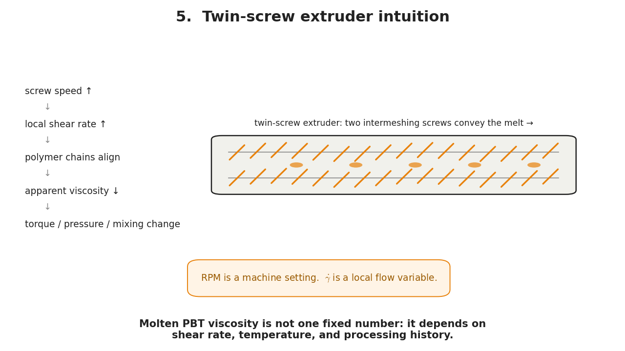
§1. Shear, and three quantities
Picture a fluid between two parallel plates. The bottom plate is fixed. The top plate is pulled sideways. The layer touching the top moves fastest; the layer near the bottom barely moves. So neighboring layers slide past one another. That sliding is shear.
Three quantities describe it. The shear stress $\tau$ is force per unit area $[\mathrm{Pa}]$ — how hard we push to deform the material. The shear rate $\dot{\gamma}$ is the velocity gradient $[\mathrm{s}^{-1}]$; for a planar profile $u(y)$, $$ \dot{\gamma}=\frac{du}{dy}. $$ The viscosity $\eta$ is resistance to flow $[\mathrm{Pa\cdot s}]$, defined in simple shear by $\eta=\tau/\dot{\gamma}$.
§2. Newtonian fluids: one constant viscosity
The simplest idealization is the Newtonian law: stress is proportional to shear rate.
$$ \tau=\eta\,\dot{\gamma},\qquad \eta=\text{const at fixed }T,\,p,\text{ composition.} $$
Double the shear rate and you double the stress. Water and simple solvents are approximately Newtonian under ordinary conditions.
Newtonian does not mean the stress stays the same. The stress still rises with
shear rate. What stays fixed is the ratio $\tau/\dot{\gamma}$. That ratio is the
viscosity.
§3. Non-Newtonian fluids: shear thinning
A non-Newtonian fluid does not obey $\tau=\eta\dot{\gamma}$ with constant $\eta$. Instead the apparent viscosity depends on the flow itself, $\eta_{\mathrm{app}}=\eta_{\mathrm{app}}(\dot{\gamma})$.
Polymer melts are usually non-Newtonian, and the reason is molecular. A melt is a tangle of long chains. At low shear the chains are entangled and randomly oriented. At higher shear the flow orients and stretches them, so they slide past each other more easily. The material offers less resistance. This is shear thinning: $$ \frac{d\eta_{\mathrm{app}}}{d\dot{\gamma}}<0. $$
§4. The power-law model
The standard first model is the Ostwald–de Waele power law. Dividing by $\dot{\gamma}$ turns the stress law into a viscosity law.
$$ \tau=K\dot{\gamma}^{\,n},\qquad
\eta_{\mathrm{app}}(\dot{\gamma})=\frac{\tau}{\dot{\gamma}}=K\dot{\gamma}^{\,n-1}. $$
Here $K$ is the consistency index and $n$ the flow-behavior index. The sign of $n-1$ decides everything.
If $n=1$, then $\eta_{\mathrm{app}}=K$ is constant: Newtonian. If $0<n<1$, then $n-1<0$, so $\eta_{\mathrm{app}}$ falls as $\dot{\gamma}$ rises: shear thinning. If $n>1$, viscosity rises with shear rate: shear thickening.
A melt typically has $0<n<1$. Take $n=\tfrac12$, so $\eta_{\mathrm{app}}=K\dot{\gamma}^{-1/2}$. Then raising the shear rate by $100$ drops the apparent viscosity by $10$. That is a power-law drop, not an exponential one.
§5. Temperature dependence
Viscosity also falls with temperature, because molecular motion becomes easier. A common local model is Arrhenius, $\eta(T)=A\exp(E_a/RT)$, with $T$ in absolute Kelvin. Because $T$ sits in the denominator, raising $T$ shrinks the exponent and lowers $\eta$.
Combining the two effects, and normalizing the Arrhenius factor about a reference temperature $T_{\mathrm{ref}}$, gives the model used in the animation:
$$ \eta_{\mathrm{app}}(\dot{\gamma},T)
=K_{\mathrm{ref}}\,
\exp\!\left[\frac{E_a}{R}\left(\frac{1}{T}-\frac{1}{T_{\mathrm{ref}}}\right)\right]
\dot{\gamma}^{\,n-1}. $$
Two leading trends: higher shear rate lowers viscosity when $n<1$, and higher temperature lowers viscosity. This is a pedagogical form, not a calibrated fit to any real PBT grade.
§6. PBT in a twin-screw extruder
Molten PBT is not water. Its viscosity is not a single number but a process-dependent quantity $\eta_{\mathrm{app}}(\dot{\gamma},T)$. In a twin-screw extruder the screws create complicated local flow fields. The local shear rate depends on screw speed, screw geometry, channel depth, gap size, fill level, and pressure.
RPM is not shear rate. Screw RPM is a machine setting. $\dot{\gamma}$ is a local
physical variable inside the flowing melt. Raising RPM usually raises typical shear rates, which
— for a shear-thinning melt — lowers apparent viscosity and makes the material easier
to convey, mix, and pump.
The response is a coupled chain: $$ \text{screw speed}\;\to\;\dot{\gamma}\;\to\;\eta_{\mathrm{app}}\;\to\; \text{pressure, torque, mixing, residence time, heat.} $$ For a Newtonian fluid, changing $\dot{\gamma}$ changes the stress but not the viscosity. For a shear-thinning melt, it changes both. That is why an extruder is a coupled thermomechanical system, not merely a liquid pump.
§7. The takeaway
Newtonian: $\tau=\eta\dot{\gamma}$ with constant $\eta$. Polymer melt: $\tau=K\dot{\gamma}^{\,n}$,
$\eta_{\mathrm{app}}=K\dot{\gamma}^{\,n-1}$, $0<n<1$. The viscosity of molten PBT is an apparent,
process-dependent quantity — specify it together with shear rate, temperature, and grade.
Python source for the animation (numpy + matplotlib + pillow; ffmpeg optional)
"""
Rheology intro animation: Newtonian fluid vs. shear-thinning polymer melt (PBT-like).

Companion to entries/mathematics/rheology-pbt-extrusion.html.
Run: python3 create_rheology_gif.py   (writes GIF / PNG / optional MP4 alongside this file)

------------------------------------------------------------------------------
The physics this animation teaches
------------------------------------------------------------------------------
Rheology studies how materials deform and flow under applied stress. In simple
shear a material is sheared between two plates; we track three quantities:

    tau      shear stress     [Pa]      force per unit area
    gdot     shear rate       [1/s]     du/dy, the velocity gradient
    eta      viscosity        [Pa s]    resistance to flow, eta = tau / gdot

Newtonian fluid (water, simple solvents at fixed T):

    tau = eta * gdot,        eta = constant.

So tau grows LINEARLY with gdot and the ratio tau/gdot never changes.

Shear-thinning polymer melt (Ostwald-de Waele power law):

    tau = K * gdot**n,       eta_app(gdot) = tau / gdot = K * gdot**(n-1).

For 0 < n < 1 the exponent n-1 < 0, so apparent viscosity DECREASES as the
shear rate increases. Molecularly: long entangled chains orient with the flow
at high shear, offering less resistance. This is a POWER-LAW drop, not an
exponential one.

Temperature: viscosity also drops with temperature. We use a normalized
Arrhenius-type factor about a reference temperature T_ref,

    eta_app(gdot, T) = K_ref * exp[ (Ea/R) * (1/T - 1/T_ref) ] * gdot**(n-1).

This is a PEDAGOGICAL model. The constants below are illustrative, not a
calibrated fit to any real PBT grade.
"""

import numpy as np
import matplotlib

matplotlib.use("Agg")  # headless: render frames without a display
import matplotlib.pyplot as plt
from matplotlib.patches import FancyArrowPatch, Rectangle, Circle, FancyBboxPatch
from matplotlib.animation import FuncAnimation, PillowWriter

try:
    from matplotlib.animation import FFMpegWriter
except Exception:  # pragma: no cover - extremely rare
    FFMpegWriter = None

from pathlib import Path

# --------------------------------------------------------------------------
# Pedagogical material parameters (NOT a calibrated PBT fit)
# --------------------------------------------------------------------------
K_ref = 1000.0          # Pa s^n, consistency index at T_ref
n = 0.45                # shear-thinning index, 0 < n < 1
eta_newtonian = 300.0   # Pa s, constant Newtonian viscosity
Ea = 50_000.0           # J/mol, apparent activation energy for flow
R = 8.314               # J/(mol K), gas constant
T_ref = 533.15          # K  (~260 C), reference temperature
T_cold = 513.15         # K  (~240 C)
T_hot = 553.15          # K  (~280 C)

# Shear-rate axis: log-spaced over [1e-1, 1e3] s^-1
GDOT = np.logspace(-1, 3, 400)


# --------------------------------------------------------------------------
# Rheological model functions
# --------------------------------------------------------------------------
def eta_polymer(gdot, T):
    """Apparent viscosity of the polymer melt, eta_app(gdot, T) [Pa s].

    Power-law shear thinning times a normalized Arrhenius temperature factor.
    """
    arrhenius = np.exp(Ea / R * (1.0 / T - 1.0 / T_ref))
    return K_ref * arrhenius * gdot ** (n - 1.0)


def tau_polymer(gdot, T):
    """Shear stress of the polymer melt, tau = eta_app * gdot [Pa]."""
    return eta_polymer(gdot, T) * gdot


def tau_newtonian(gdot):
    """Newtonian shear stress, tau = eta * gdot [Pa]."""
    return eta_newtonian * gdot


# --------------------------------------------------------------------------
# Color palette (<= 4 main colors) and global style
# --------------------------------------------------------------------------
C_NEWT = "#1f6fb2"   # Newtonian: blue
C_POLY = "#e8820c"   # polymer melt (reference T): orange
C_COLD = "#5e3c99"   # cold curve: purple
C_HOT = "#d7301f"    # hot curve: red
C_INK = "#222222"    # text / structure
C_FAINT = "#888888"

plt.rcParams.update({
    "font.size": 15,
    "font.family": "DejaVu Sans",
    "axes.titlesize": 17,
    "axes.labelsize": 16,
    "axes.edgecolor": "#444444",
    "xtick.labelsize": 12,
    "ytick.labelsize": 12,
    "mathtext.fontset": "cm",
    "figure.facecolor": "white",
    "axes.facecolor": "white",
    "savefig.facecolor": "white",
})


# --------------------------------------------------------------------------
# Frame / scene bookkeeping
# --------------------------------------------------------------------------
fps = 12
duration_sec = 16
n_frames = fps * duration_sec            # 192 frames
scene_edges = [0, 36, 72, 120, 156, 192] # scene boundaries in frames


def scene_progress(frame, start, end):
    """Fractional progress in [0,1] of `frame` within scene [start, end)."""
    return np.clip((frame - start) / (end - start), 0.0, 1.0)


def smoothstep(x):
    """Smooth 0->1 ease (zero slope at both ends)."""
    x = np.clip(x, 0.0, 1.0)
    return x * x * (3.0 - 2.0 * x)


# --------------------------------------------------------------------------
# Figure scaffold: a single 1280x720 canvas reused for every frame.
# We use one full-canvas axes for drawings/text and add plot axes per scene.
# --------------------------------------------------------------------------
DPI = 100
fig = plt.figure(figsize=(12.8, 7.2), dpi=DPI)

# Background axes covering the whole figure for titles, schematics, labels.
bg = fig.add_axes([0, 0, 1, 1])
bg.set_xlim(0, 1)
bg.set_ylim(0, 1)
bg.axis("off")


def _text(x, y, s, size=16, color=C_INK, ha="left", va="center",
          weight="normal", style="normal", alpha=1.0):
    """Convenience wrapper for background-axes text in figure coordinates."""
    return bg.text(x, y, s, size=size, color=color, ha=ha, va=va,
                   weight=weight, style=style, alpha=alpha, zorder=10)


# --------------------------------------------------------------------------
# Helper: simple-shear cell (two plates + sliding fluid layers)
# --------------------------------------------------------------------------
def draw_shear_cell(ax, progress, mode="newtonian"):
    """Draw a sheared fluid between a fixed bottom plate and a moving top plate.

    progress in [0,1] animates the top plate sliding right and the per-layer
    velocity arrows growing (longer near the top: a linear velocity gradient).
    `mode` only sets the accent color of the fluid block.
    """
    ax.clear()
    ax.set_xlim(0, 10)
    ax.set_ylim(0, 10)
    ax.axis("off")

    accent = C_NEWT if mode == "newtonian" else C_POLY
    x0, x1 = 1.2, 8.0
    y_bot, y_top = 2.0, 8.0
    shift = 1.6 * progress  # how far the top plate has slid

    # Fluid block (light fill) -- the sheared material.
    ax.add_patch(Rectangle((x0, y_bot), x1 - x0, y_top - y_bot,
                           facecolor=accent, alpha=0.10,
                           edgecolor="none", zorder=1))

    # Fixed bottom plate (hatched bar) and moving top plate.
    ax.add_patch(Rectangle((x0 - 0.3, y_bot - 0.45), x1 - x0 + 0.6, 0.45,
                           facecolor="#cfcfcf", edgecolor=C_INK, zorder=3))
    ax.add_patch(Rectangle((x0 - 0.3 + shift, y_top), x1 - x0 + 0.6, 0.45,
                           facecolor="#cfcfcf", edgecolor=C_INK, zorder=3))

    # Fluid layers: horizontal lines that skew with height (top moves most).
    n_layers = 7
    for i in range(n_layers):
        frac = i / (n_layers - 1)              # 0 at bottom, 1 at top
        y = y_bot + frac * (y_top - y_bot)
        dx = shift * frac                       # linear velocity profile
        ax.plot([x0 + dx, x1 + dx], [y, y], color=accent, lw=1.4,
                alpha=0.55, zorder=2)
        # Velocity arrow: length grows with height -> shear rate = du/dy.
        arrow_len = 0.25 + 2.4 * frac * (0.4 + 0.6 * progress)
        if arrow_len > 0.05:
            ax.add_patch(FancyArrowPatch(
                (x1 + dx + 0.15, y), (x1 + dx + 0.15 + arrow_len, y),
                arrowstyle="-|>", mutation_scale=12,
                color=accent, lw=2.0, zorder=4))

    # Annotate the moving / fixed plates.
    ax.text((x0 + x1) / 2 + shift, y_top + 0.7, "top plate moves  →",
            ha="center", va="bottom", fontsize=12.5, color=C_INK)
    ax.text((x0 + x1) / 2, y_bot - 0.95, "fixed bottom plate",
            ha="center", va="top", fontsize=12.5, color=C_INK)
    # Velocity-gradient bracket label.
    ax.text(x1 + 1.9, (y_bot + y_top) / 2,
            r"$u(y)$" "\n" r"$\dot{\gamma}=du/dy$",
            ha="left", va="center", fontsize=13, color=accent)


# --------------------------------------------------------------------------
# Helper: cartoon polymer chains, oriented by `alignment` in [0,1]
# --------------------------------------------------------------------------
def draw_polymer_chains(ax, alignment, seed=0):
    """Draw squiggly polymer chains; alignment 0 = tangled, 1 = flow-aligned.

    Each chain is a sine squiggle with a random phase. At low alignment the
    chains take random orientations; at high alignment they rotate toward the
    horizontal (flow) direction and stretch out, the molecular picture behind
    shear thinning.
    """
    ax.clear()
    ax.set_xlim(0, 10)
    ax.set_ylim(0, 10)
    ax.axis("off")

    a = smoothstep(alignment)
    rng = np.random.default_rng(seed)  # fixed seed -> stable chains across frames
    n_chains = 9
    t = np.linspace(-1.0, 1.0, 60)

    for _ in range(n_chains):
        cx = rng.uniform(1.8, 8.2)
        cy = rng.uniform(2.0, 8.0)
        length = (1.1 + 0.4 * rng.random()) * (1.0 + 0.9 * a)   # stretch out
        amp = (0.45 + 0.35 * rng.random()) * (1.0 - 0.75 * a)   # uncrinkle
        phase = rng.uniform(0, 2 * np.pi)
        waves = rng.uniform(2.0, 3.5)

        # Local chain shape: a stretched axis (xs) + transverse squiggle (ys).
        xs = length * t
        ys = amp * np.sin(waves * np.pi * t + phase)

        # Orientation: random when tangled, -> horizontal as it aligns.
        theta0 = rng.uniform(0, 2 * np.pi)
        theta = (1.0 - a) * theta0  # collapse toward 0 rad (flow direction)
        ct, st = np.cos(theta), np.sin(theta)
        X = cx + ct * xs - st * ys
        Y = cy + st * xs + ct * ys

        ax.plot(X, Y, color=C_POLY, lw=2.2, alpha=0.85, solid_capstyle="round")

    # Flow-direction velocity arrows, growing with alignment (= shear rate).
    for yk in (3.0, 5.0, 7.0):
        L = 0.6 + 2.4 * a
        ax.add_patch(FancyArrowPatch((0.6, yk), (0.6 + L, yk),
                                     arrowstyle="-|>", mutation_scale=12,
                                     color=C_FAINT, lw=1.8))


# --------------------------------------------------------------------------
# Helper: simplified twin-screw extruder schematic
# --------------------------------------------------------------------------
def draw_extruder(ax, progress):
    """Two intermeshing rotating screws in a barrel; melt moves left to right."""
    ax.clear()
    ax.set_xlim(0, 10)
    ax.set_ylim(0, 10)
    ax.axis("off")

    bx0, bx1, by0, by1 = 0.6, 9.4, 3.2, 6.8

    # Barrel outline.
    ax.add_patch(FancyBboxPatch((bx0, by0), bx1 - bx0, by1 - by0,
                                boxstyle="round,pad=0.02,rounding_size=0.25",
                                facecolor="#f1f1ec", edgecolor=C_INK, lw=1.8,
                                zorder=1))

    # Two screw shafts drawn as a series of flights (slanted ticks) that
    # appear to rotate/convey as `progress` advances.
    phase = 2 * np.pi * progress
    for cy in (by0 + 1.0, by1 - 1.0):
        ax.plot([bx0 + 0.4, bx1 - 0.4], [cy, cy], color=C_FAINT, lw=1.2,
                zorder=2)
        nf = 16
        for k in range(nf):
            xf = bx0 + 0.6 + (bx1 - bx0 - 1.2) * k / (nf - 1)
            s = 0.5 * np.sin(phase + k * 0.9)   # flight tilt animates
            ax.plot([xf - 0.18, xf + 0.18], [cy - 0.45 + s * 0.25,
                                              cy + 0.45 + s * 0.25],
                    color=C_POLY, lw=2.4, solid_capstyle="round", zorder=3)

    # Melt moving left -> right: a few markers advancing with progress.
    for j in range(5):
        mx = bx0 + 0.8 + ((j / 5.0 + progress) % 1.0) * (bx1 - bx0 - 1.6)
        ax.add_patch(Circle((mx, (by0 + by1) / 2), 0.16,
                            facecolor=C_POLY, edgecolor="none",
                            alpha=0.7, zorder=4))

    ax.text((bx0 + bx1) / 2, by1 + 0.5,
            "twin-screw extruder: two intermeshing screws convey the melt →",
            ha="center", va="bottom", fontsize=12.5, color=C_INK)


# --------------------------------------------------------------------------
# Helper: clean up a Matplotlib plot axis (spines, grid)
# --------------------------------------------------------------------------
def setup_clean_axis(ax):
    ax.spines["top"].set_visible(False)
    ax.spines["right"].set_visible(False)
    ax.grid(True, which="both", color="#dddddd", lw=0.6, alpha=0.7)
    ax.set_axisbelow(True)


def save_last_frame(fig, filename):
    """Save the current figure state as a PNG poster of the final frame."""
    fig.savefig(filename, dpi=DPI)


# --------------------------------------------------------------------------
# Per-scene renderers. Each receives local progress p in [0,1].
# We create/destroy plot axes per frame so the single canvas can morph.
# --------------------------------------------------------------------------
# Track dynamically-added axes so we can clear them each frame.
_dyn_axes = []


def _clear_dynamic():
    for ax in _dyn_axes:
        ax.remove()
    _dyn_axes.clear()
    bg.clear()
    bg.set_xlim(0, 1)
    bg.set_ylim(0, 1)
    bg.axis("off")


def _header(title, subtitle=None):
    _text(0.5, 0.95, title, size=22, ha="center", weight="bold")
    if subtitle:
        _text(0.5, 0.895, subtitle, size=14, ha="center", color=C_FAINT)


def scene1(p):
    """What is shear? Animated plates + growing velocity arrows."""
    _header("1.  What is shear?")
    ax = fig.add_axes([0.05, 0.08, 0.62, 0.74]); _dyn_axes.append(ax)
    draw_shear_cell(ax, smoothstep(p), mode="newtonian")

    _text(0.70, 0.70,
          "Shear = neighboring layers\nsliding past one another",
          size=15)
    _text(0.70, 0.50,
          r"Shear rate  $\dot{\gamma}$:  speed gradient",
          size=15, color=C_NEWT)
    _text(0.70, 0.38,
          r"Shear stress  $\tau$:  force per area",
          size=15, color=C_NEWT)
    _text(0.70, 0.22, r"$\eta = \tau/\dot{\gamma}$  (viscosity)",
          size=16)


def scene2(p):
    """Newtonian fluid: tau = eta * gdot, linear, marker sweeps the line."""
    _header("2.  Newtonian fluid", r"$\tau = \eta\,\dot{\gamma}$,   $\eta$ constant")

    # Left: shear cell.
    axL = fig.add_axes([0.03, 0.08, 0.40, 0.70]); _dyn_axes.append(axL)
    draw_shear_cell(axL, 1.0, mode="newtonian")

    # Right: tau vs gdot on LINEAR axes.
    axR = fig.add_axes([0.55, 0.16, 0.40, 0.64]); _dyn_axes.append(axR)
    setup_clean_axis(axR)
    g = np.linspace(0, 1000, 200)
    axR.plot(g, tau_newtonian(g), color=C_NEWT, lw=3)
    axR.set_xlabel(r"$\dot{\gamma}\ \mathrm{(s^{-1})}$")
    axR.set_ylabel(r"$\tau\ \mathrm{(Pa)}$")
    axR.set_xlim(0, 1000)
    axR.set_ylim(0, tau_newtonian(1000) * 1.05)

    # Marker sweeping along the line as gdot increases.
    gm = 1000 * smoothstep(p)
    axR.plot([gm], [tau_newtonian(gm)], "o", color=C_NEWT, ms=11,
             markeredgecolor="white")
    axR.text(0.05, 0.90,
             r"$\eta=\tau/\dot{\gamma}=300\ \mathrm{Pa\,s}$ (fixed)",
             transform=axR.transAxes, fontsize=13, color=C_NEWT)

    _text(0.5, 0.045,
          "Double the shear rate, double the stress.  The ratio stays fixed.",
          size=15, ha="center")


def scene3(p):
    """Polymer melt: chains align (left) + log-log eta drop (right)."""
    _header("3.  Polymer melt: chains align, viscosity drops")

    a = smoothstep(p)  # alignment / marker position driver

    # Left: polymer chains becoming aligned.
    axL = fig.add_axes([0.03, 0.10, 0.40, 0.66]); _dyn_axes.append(axL)
    draw_polymer_chains(axL, a, seed=3)
    if a < 0.5:
        _text(0.23, 0.085,
              "low shear: chains tangled;\nhigh apparent viscosity",
              size=13, ha="center", color=C_POLY)
    else:
        _text(0.23, 0.085,
              "higher shear: chains align;\napparent viscosity drops",
              size=13, ha="center", color=C_POLY)

    # Right: eta_app vs gdot on LOG-LOG axes.
    axR = fig.add_axes([0.55, 0.17, 0.40, 0.60]); _dyn_axes.append(axR)
    setup_clean_axis(axR)
    axR.set_xscale("log"); axR.set_yscale("log")
    axR.plot(GDOT, eta_polymer(GDOT, T_ref), color=C_POLY, lw=3,
             label="polymer melt")
    axR.plot(GDOT, np.full_like(GDOT, eta_newtonian), color=C_NEWT, lw=2.5,
             ls="--", label="Newtonian")
    axR.set_xlabel(r"$\dot{\gamma}\ \mathrm{(s^{-1})}$")
    axR.set_ylabel(r"$\eta_{\mathrm{app}}\ \mathrm{(Pa\cdot s)}$")
    axR.set_ylim(10, 1e4)
    # Direct labels (no tiny legend).
    axR.text(2e2, eta_newtonian * 1.25, "Newtonian  $\\eta=300$",
             color=C_NEWT, fontsize=12, ha="center")
    axR.text(2e0, eta_polymer(2e0, T_ref) * 1.5,
             r"$\eta_{\mathrm{app}}=K\dot{\gamma}^{\,n-1}$",
             color=C_POLY, fontsize=13)

    # Marker sweeping from low to high gdot along the polymer curve.
    gm = 10 ** (-1 + 4 * a)
    axR.plot([gm], [eta_polymer(gm, T_ref)], "o", color=C_POLY, ms=11,
             markeredgecolor="white", zorder=5)

    _text(0.5, 0.05,
          r"$0<n<1$:  power-law drop, not exponential drop.",
          size=15, ha="center")


def scene4(p):
    """Temperature effect: cold / ref / hot curves; hot animates in lower."""
    _header("4.  Temperature lowers viscosity")

    ax = fig.add_axes([0.30, 0.16, 0.45, 0.60]); _dyn_axes.append(ax)
    setup_clean_axis(ax)
    ax.set_xscale("log"); ax.set_yscale("log")
    ax.set_xlabel(r"$\dot{\gamma}\ \mathrm{(s^{-1})}$")
    ax.set_ylabel(r"$\eta_{\mathrm{app}}\ \mathrm{(Pa\cdot s)}$")
    ax.set_ylim(10, 3e4)

    a = smoothstep(p)
    # Cold and reference are drawn immediately; the hot curve fades/drops in.
    ax.plot(GDOT, eta_polymer(GDOT, T_cold), color=C_COLD, lw=3)
    ax.plot(GDOT, eta_polymer(GDOT, T_ref), color=C_POLY, lw=3)
    ax.plot(GDOT, eta_polymer(GDOT, T_hot), color=C_HOT, lw=3, alpha=a)

    # Direct curve labels.
    ax.text(1.2e-1, eta_polymer(1.2e-1, T_cold) * 1.05,
            r"cold $240^\circ$C", color=C_COLD, fontsize=12.5)
    ax.text(1.2e-1, eta_polymer(1.2e-1, T_ref) * 1.05,
            r"ref $260^\circ$C", color=C_POLY, fontsize=12.5)
    ax.text(1.2e-1, eta_polymer(1.2e-1, T_hot) * 0.78,
            r"hot $280^\circ$C", color=C_HOT, fontsize=12.5, alpha=a)

    _text(0.5, 0.86,
          r"$\eta_{\mathrm{app}}(\dot{\gamma},T)=K_{\mathrm{ref}}\,"
          r"\exp\!\left[\frac{E_a}{R}\left(\frac{1}{T}-\frac{1}{T_{\mathrm{ref}}}"
          r"\right)\right]\dot{\gamma}^{\,n-1}$",
          size=15, ha="center")
    _text(0.5, 0.06,
          "Higher temperature usually lowers melt viscosity.",
          size=15, ha="center")


def scene5(p):
    """Twin-screw extruder intuition + causal chain + final takeaway."""
    _header("5.  Twin-screw extruder intuition")

    ax = fig.add_axes([0.30, 0.30, 0.66, 0.46]); _dyn_axes.append(ax)
    draw_extruder(ax, p)

    # Causal chain on the left.
    chain = [
        "screw speed ↑",
        "local shear rate ↑",
        "polymer chains align",
        "apparent viscosity ↓",
        "torque / pressure / mixing change",
    ]
    y = 0.74
    for i, line in enumerate(chain):
        shown = smoothstep(scene_progress(p, i * 0.12, i * 0.12 + 0.25))
        _text(0.04, y, line, size=13.5, color=C_INK, alpha=shown)
        if i < len(chain) - 1:
            _text(0.07, y - 0.045, "↓", size=13, color=C_FAINT,
                  alpha=shown)
        y -= 0.095

    # Caution box.
    bg.add_patch(FancyBboxPatch((0.31, 0.165), 0.40, 0.085,
                                boxstyle="round,pad=0.01,rounding_size=0.02",
                                transform=bg.transAxes,
                                facecolor="#fff4e6", edgecolor=C_POLY,
                                lw=1.4, zorder=9))
    _text(0.51, 0.207,
          r"RPM is a machine setting.  $\dot{\gamma}$ is a local flow variable.",
          size=13.5, ha="center", color="#9a5a00")

    # Final takeaway.
    _text(0.5, 0.06,
          "Molten PBT viscosity is not one fixed number: it depends on\n"
          "shear rate, temperature, and processing history.",
          size=15, ha="center", weight="bold")


# --------------------------------------------------------------------------
# Master frame dispatcher
# --------------------------------------------------------------------------
def render_frame(frame):
    _clear_dynamic()
    if frame < scene_edges[1]:
        scene1(scene_progress(frame, scene_edges[0], scene_edges[1]))
    elif frame < scene_edges[2]:
        scene2(scene_progress(frame, scene_edges[1], scene_edges[2]))
    elif frame < scene_edges[3]:
        scene3(scene_progress(frame, scene_edges[2], scene_edges[3]))
    elif frame < scene_edges[4]:
        scene4(scene_progress(frame, scene_edges[3], scene_edges[4]))
    else:
        scene5(scene_progress(frame, scene_edges[4], scene_edges[5]))
    return []


def main():
    here = Path(__file__).parent
    gif_path = here / "rheology_pbt_intro.gif"
    mp4_path = here / "rheology_pbt_intro.mp4"
    png_path = here / "rheology_pbt_intro_last_frame.png"

    anim = FuncAnimation(fig, render_frame, frames=n_frames, blit=False)

    # --- GIF (always) ---
    anim.save(str(gif_path), writer=PillowWriter(fps=fps))
    print("Created rheology_pbt_intro.gif")

    # --- MP4 (only if ffmpeg is available) ---
    mp4_ok = False
    if FFMpegWriter is not None and FFMpegWriter.isAvailable():
        try:
            anim.save(str(mp4_path), writer=FFMpegWriter(fps=fps, bitrate=2400))
            mp4_ok = True
            print("Created rheology_pbt_intro.mp4")
        except Exception as exc:  # pragma: no cover
            print(f"MP4 skipped because ffmpeg failed: {exc}")
    if not mp4_ok and not mp4_path.exists():
        print("MP4 skipped because ffmpeg is unavailable.")

    # --- Last frame as PNG poster ---
    render_frame(n_frames - 1)
    save_last_frame(fig, str(png_path))
    print("Created rheology_pbt_intro_last_frame.png")


if __name__ == "__main__":
    main()
The Ostwald–de Waele power law $\tau=K\dot{\gamma}^{n}$ (hence $\eta_{\mathrm{app}}=K\dot{\gamma}^{n-1}$) and the Arrhenius temperature factor are standard introductory rheology. The constants here ($K_{\mathrm{ref}}$, $n=0.45$, $E_a$, $T_{\mathrm{ref}}\approx260^\circ$C) are illustrative values chosen for a clean visualization, not a material fit to a specific PBT grade. Companion code: code/rheology_pbt/create_rheology_gif.py.
Replay: iCaRL and generative rehearsal
Replay preserves old knowledge by revisiting past data — either stored exemplars or samples synthesized by a generator. It is the family that holds up best in Class-IL. I take iCaRL as the canonical exemplar method, make its stagewise update precise, and show why exemplar quality controls how close it gets to the ideal nearest-mean classifier. Then I turn to generative rehearsal, which replaces the buffer with a model and is the bridge to the diffusion entries.
§1. iCaRL: what is stored, and the update
iCaRL trains incrementally on batches of classes; after each batch the classifier is evaluated only on classes seen so far.1 Two things define it: what sits in the buffer, and the update rule. Consider class-incremental stages $b=1,\dots,B$. At stage $b$ a batch of new classes $\c{N}_b$ arrives with data $\c{D}_b^{\mathrm{new}}=\crbr{(x_i,y_i)}_{i=1}^{n_b}$, $y_i\in\c{N}_b$, and $\c{C}_b=\bigcup_{r\le b}\c{N}_r$ is everything seen so far. The state is $$ S_b=(\Theta_b,\,W_b,\,P^{(b)}), \qquad \phi_{\Theta_b}:\c{X}\to\RR^d, $$ a feature extractor $\phi_{\Theta_b}$, class output weights $W_b$, and an exemplar memory $P^{(b)}=(P_y^{(b)})_{y\in\c{C}_b}$ obeying the budget $\sum_{y\in\c{C}_b}|P_y^{(b)}|\le K$. The update map has input $(S_{b-1},\c{D}_b^{\mathrm{new}},K)$ and output $S_b$ plus a deployed classifier $f_b:\c{X}\to\c{C}_b$. The objective is not just to fit new classes but to keep high accuracy on all of $\c{C}_b$ under the fixed budget $K$.
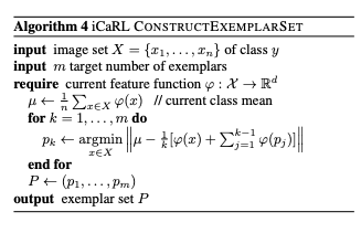
Herding: exemplars $p_1,\dots,p_m$ are added one at a time, each chosen so the running mean of stored features best approximates the mean feature over all training examples.
§2. Incremental representation update
Suppose stage $b$ adds classes $C_b=\crbr{s,\dots,t}$, with previous parameters $\Theta^{\mathrm{old}}$ and exemplars $P^{\mathrm{old}}=(P_1,\dots,P_{s-1})$. Form the rehearsal set $$ \widetilde D_b = \bigcup_{y=s}^{t}\crbr{(x,y):x\in X_y}\ \cup\ \bigcup_{y=1}^{s-1}\crbr{(x,y):x\in P_y}. $$ For each sample and each old class $y\le s-1$ store the pre-update score $q_{i,y}:=g_y^{\mathrm{old}}(x_i)$, then update $\Theta$ by minimizing $$ \c{L}_b(\Theta) = \sum_{(x_i,y_i)\in\widetilde D_b}\smbr{\sum_{y=s}^{t}\operatorname{BCE}\!\smbr{\mathbf 1\crbr{y_i=y},g_y(x_i)} + \sum_{y=1}^{s-1}\operatorname{BCE}\!\smbr{q_{i,y},g_y(x_i)}}. $$ The first sum learns the new classes; the second distills the old responses so the representation does not drift too violently. Afterward the budget is rebalanced uniformly, $m_b=\lfloor K/|\c{C}_b|\rfloor$: old exemplar sets are truncated to $m_b$, each new class gets a prioritized list of length $m_b$. A standard summary is the average incremental accuracy $\overline A_B=\tfrac1B\sum_b A_b$.
§3. Why exemplar quality matters: an NCM bound
Read iCaRL against the ideal nearest-class-mean (NCM) classifier.2 Let $m_y=\tfrac1{|X_y|}\sum_{x\in X_y}\phi_\Theta(x)$ be the true class mean and $\mu_y=\tfrac1{|P_y|}\sum_{p\in P_y}\phi_\Theta(p)$ the exemplar mean iCaRL actually uses. Because features are normalized, the decision rule $y^*(x)=\arg\min_y\|\phi_\Theta(x)-\mu_y\|_2$ equals $\arg\max_y\mu_y^\top\phi_\Theta(x)$. With NCM score $s_y(x)=m_y^\top\phi_\Theta(x)$, iCaRL score $\hat s_y(x)=\mu_y^\top\phi_\Theta(x)$, and $\varepsilon=\max_y\|\mu_y-m_y\|_2$, Cauchy–Schwarz gives $$ |\hat s_y(x)-s_y(x)| = |(\mu_y-m_y)^\top\phi_\Theta(x)| \le \|\mu_y-m_y\|_2\,\|\phi_\Theta(x)\|_2 \le \varepsilon. $$
Hence if $c$ is correct and the NCM margin satisfies
$s_c(x)-\max_{y\neq c}s_y(x) > 2\varepsilon$, then iCaRL and NCM predict the same label.
This is not stated in the original paper, but it makes precise why exemplar selection matters: small prototype error $\varepsilon$ ⇒ iCaRL behaves like ideal NCM on every point whose margin is not too small. Distillation plays a different role — it does not bound $\varepsilon$ directly but controls representation drift so old-class discrimination is not destroyed.1,3 Later work re-reads iCaRL: Javed & Shafait argue distillation, not herding, is the dominant factor; BiC/WA/LUCIR/PODNet rectify old-new bias and strengthen the representation; GDumb shows simple replay can be surprisingly strong; and the modern frontier splits between analytic methods (ACIL) and pretrained-backbone methods (SimpleCIL, etc.). iCaRL is best seen as the foundational replay-distillation baseline.4
§4. Generative rehearsal
When storing real data is undesirable, replace the buffer with a model — Robins' pseudorehearsal, realized for deep nets as deep generative replay.5 The biological motivation is the complementary learning systems (CLS) theory: a fast-learning hippocampus and a slow-learning neocortex, with reactivation that is flexible rather than a literal replay buffer.
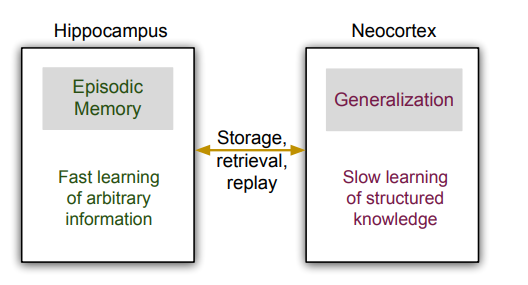
Complementary learning systems: hippocampus for fast episodic learning, neocortex for slow structured knowledge.6
Generative replay (one task at a time). Keep a current generator
$G_{\mathrm{curr}}$ and a frozen copy $G_{\mathrm{frozen}}$.
- Task $0$: train $G_{\mathrm{curr}}$ on real data $D_0$ only.
- Task $t>0$: until converged, sample real $x_{\mathrm{real}}\sim D_t$ and synthetic past $x_{\mathrm{past}}\sim G_{\mathrm{frozen}}(z)$, train $G_{\mathrm{curr}}$ on $x_{\mathrm{real}}\cup x_{\mathrm{past}}$.
- Set $G_{\mathrm{frozen}}\leftarrow\operatorname{Copy}(G_{\mathrm{curr}})$.
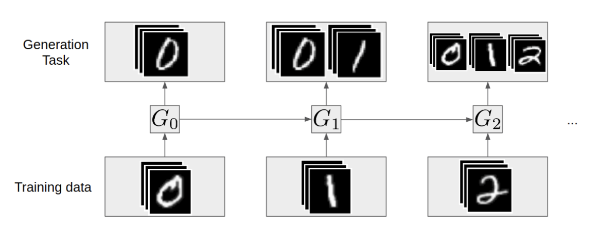
$G_0$ trains on real ‘0’s; the frozen copy then feeds ‘0’s into $G_1$ alongside real ‘1’s, so $G_1$ generates both, and so on. Image quality is tracked by FID (§5).7
Lesort et al. asked which CL algorithm works best on which generative model.7 Their conclusion: rehearsal is effective and stable for VAE / CVAE (a probabilistic latent and pixel-wise loss make them less prone to overfitting a tiny stored set), but unsatisfactory and unstable for GAN variants (CGAN, WGAN-GP), where a few stored samples make the discriminator's job trivial. A related Bayesian route is variational continual learning.8
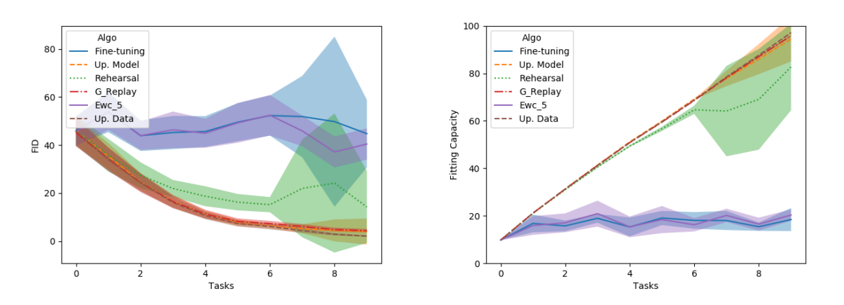
CL algorithms over 10 disjoint tasks on a GAN trained on MNIST, scored by FID (left, lower-better) and Fitting Capacity (right, higher-better) at the end of each task: $G_t$ must generate every category seen from task $0$ to $t$.
§5. Two evaluation notions
Fréchet Inception Distance (FID) compares generated and real images as Gaussians in a fixed feature space (Inception-v3 activations, typically $2048$-dim): $$ \mathrm{FID} = \|\mu_r-\mu_g\|^2 + \operatorname{Tr}\!\smbr{\Sigma_r+\Sigma_g-2(\Sigma_r\Sigma_g)^{1/2}}. $$ The first term is mean shift, the second covariance mismatch; perfect mimicry gives $\mu_r\approx\mu_g$, $\Sigma_r\approx\Sigma_g$, and $\mathrm{FID}\approx 0$. (Worked examples and the MMD/KID generalization live in the metrics entry.)
Fitting capacity measures usefulness rather than appearance. Train a generator $G_\theta$, synthesize a labeled set $\c{D}_{\mathrm{gen}}=\crbr{(x_i,y_i)}$ with $x_i\sim G_\theta(z)$, fit a classifier $\phi^*=\arg\min_\phi\EE_{(x,y)\sim\c{D}_{\mathrm{gen}}}\sqbr{\c{L}(C_\phi(x),y)}$, and report its accuracy on the real test set: $$ \mathrm{FC}(G_\theta) = \EE_{(x,y)\sim\c{D}_{\mathrm{test}}}\sqbr{\mathbf 1\crbr{C_{\phi^*}(x)=y}}. $$ For an unconditional GAN one annotates synthetic images with an expert classifier first. Train-on-synthetic, test-on-real: if that classifier reaches 85% on real MNIST, the generator's fitting capacity is 85%.
1 Rebuffi et al., “iCaRL: incremental classifier and representation learning,” arXiv:1611.07725. 2 Mensink et al., IEEE TPAMI 2013. 3 Li & Hoiem, “Learning without forgetting,” ECCV 2016. 4 Javed & Shafait, ACCV 2018; Wu et al. (BiC) CVPR 2019; Hou et al. (LUCIR) CVPR 2019; Douillard et al. (PODNet) ECCV 2020; Prabhu et al. (GDumb) ECCV 2020; Zhuang et al. (ACIL) NeurIPS 2022; Zhou et al. (SimpleCIL) arXiv:2303.07338. 5 Robins, Connection Science 1995; Shin et al., “Continual learning with deep generative replay,” NeurIPS 2017. 6 McClelland, McNaughton & O'Reilly, Psych. Review 1995. 7 Lesort et al., “Generative models from the perspective of continual learning,” arXiv:1812.09111. 8 Nguyen et al., “Variational continual learning,” arXiv:1710.10628; Farquhar & Gal, “A unifying Bayesian view of continual learning,” arXiv:1902.06494. — generative rehearsal becomes diffusion-specific in algorithms; the formal problem is set up next.
$R^2$ — the coefficient of determination
$R^2$ scores a model against the laziest baseline there is: the constant that predicts the mean. We fix the definition, read it as one ratio of squared errors, and then play with it — the widget below lets you drag a line $y=mx+b$ by hand and watch $SS_{\text{res}}$ and $R^2$ respond.
§1. Definition
Fix $n$ observations $(x_i,y_i)$, write $\bar y=\tfrac1n\sum_i y_i$ for the mean of the targets, and let $\hat y_i$ be the prediction of the model under evaluation. Two sums of squares compare the model against the mean baseline:
- $SS_{\text{tot}}:\mathbb{R}^{n}\to\mathbb{R}_{\ge 0}$, the squared error of the intercept-only model $\bar y$: $$SS_{\text{tot}}=\sum_{i=1}^{n}(y_i-\bar y)^2.$$
- $SS_{\text{res}}:\mathbb{R}^{n}\times\mathbb{R}^{n}\to\mathbb{R}_{\ge 0}$, the squared error of the evaluated model $\hat y$: $$SS_{\text{res}}=\sum_{i=1}^{n}(y_i-\hat y_i)^2.$$
$R^2$ is the share of $SS_{\text{tot}}$ that the model removes — equivalently, one minus the fraction of squared error it leaves behind:
$$\boxed{\;R^2 \;=\; 1-\frac{SS_{\text{res}}}{SS_{\text{tot}}}\;}$$
The baseline scores $R^2=0$: predicting $\bar y$ everywhere gives $SS_{\text{res}}=SS_{\text{tot}}$. A perfect fit scores $R^2=1$. Nothing forces $R^2\ge 0$, though. A line worse than the mean has $SS_{\text{res}}>SS_{\text{tot}}$, hence $R^2<0$ — the widget flags this in red.
§2. By hand
Drag the two sliders to fit the prediction line $y=mx+b$ by eye. The metrics recompute on every move under the strict definition above; toggle the mean line ($\bar y$) and the residual segments $y_i-\hat y_i$ to see what each sum of squares is measuring.
Fit $y=mx+b$ by eye; watch $SS_{\text{res}}$ and $R^2$ respond. $R^2$ turns red once the line is worse than the mean baseline.
— sequel: across several tasks, averaging the per-task $R^2$ versus pooling all points into one score gives two different numbers, and the gap has a clean form: averaging vs pooling $R^2$.
Averaging vs pooling $R^2$
Score a decoder on several tasks at once and there are two honest ways to report one number, and they need not agree. Score each task on its own and average ($R_{\mathrm{all}}$), or pool every point into one pile and score once ($R_{\mathrm{pool}}$). The gap is not noise: pooling quietly enlarges the denominator by the spread between task means, so $R_{\mathrm{pool}}$ can look excellent while every per-task score sits near zero. We fix the two definitions, prove the within–between split that separates them, read the difference as two named terms, and then push the sliders. — prerequisite: the single-task definition, $R^2$.
§1. Two scores
Index tasks $d=1,\dots,D$, with $n_d$ points $\{y_{di}\}_i$ on task $d$ and predictions $\{\widehat y_{di}\}_i$. Write the task mean $\bar y_d=\tfrac1{n_d}\sum_i y_{di}$ and the two per-task sums of squares $$A_d=\sum_{i=1}^{n_d}(y_{di}-\widehat y_{di})^2,\qquad B_d=\sum_{i=1}^{n_d}(y_{di}-\bar y_d)^2\quad(B_d>0).$$ The task score is $R_d=1-A_d/B_d$ — the single-task $R^2$ of that entry, one per task. Averaging gives
$$\boxed{\;R_{\mathrm{all}}:=\frac1D\sum_{d=1}^D R_d=1-\frac1D\sum_{d=1}^D\frac{A_d}{B_d}\;}$$
Pooling instead concatenates all $N=\sum_d n_d$ points, measures them against the single pooled mean $\bar y=\tfrac1N\sum_d\sum_i y_{di}$, and scores once:
$$\boxed{\;R_{\mathrm{pool}}:=1-\frac{\sum_d A_d}{\sum_d\sum_i(y_{di}-\bar y)^2}\;}$$
One is an average of ratios; the other a single ratio. The numerator $\sum_d A_d$ — the total residual — is the same in both. Everything turns on the denominators.
§2. The within–between split
The pooled denominator is not $\sum_d B_d$; it carries an extra term.
Lemma. With $C:=\sum_d n_d(\bar y_d-\bar y)^2$ the between-task sum of squares, $$\sum_d\sum_i(y_{di}-\bar y)^2=\sum_d B_d+C, \qquad\text{hence}\qquad R_{\mathrm{pool}}=1-\frac{\sum_d A_d}{\sum_d B_d+C}.$$
Proof. Split each deviation through its task mean, $y_{di}-\bar y=(y_{di}-\bar y_d)+(\bar y_d-\bar y)$, square, and sum over $i$. The cross term carries the factor $\sum_i(y_{di}-\bar y_d)=0$ and vanishes, leaving $\sum_i(y_{di}-\bar y)^2=B_d+n_d(\bar y_d-\bar y)^2$. Sum over $d$. $\square$
$R_{\mathrm{all}}$ divides task by task; $R_{\mathrm{pool}}$ divides once, against the inflated $\sum_d B_d+C$. When the task means are well separated, $C$ dominates and the pooled denominator balloons — predicting each task's mean already “explains” the between-task gaps, for free.
§3. The gap, in two terms
The difference has a clean closed form. Write $\lambda_d=A_d/B_d$ for the per-task error ratio (so $R_d=1-\lambda_d$), two weightings of it — uniform and $B$-weighted — and the within-share $\alpha$: $$\lambda_{\mathrm{unif}}=\frac1D\sum_d\lambda_d,\qquad \lambda_B=\frac{\sum_d B_d\,\lambda_d}{\sum_d B_d},\qquad \alpha=\frac{\sum_d B_d}{\sum_d B_d+C}\in(0,1].$$ Then $R_{\mathrm{all}}=1-\lambda_{\mathrm{unif}}$; and since $\sum_d A_d=\lambda_B\sum_d B_d$ while $\sum_d B_d+C=\alpha^{-1}\sum_d B_d$, also $R_{\mathrm{pool}}=1-\alpha\lambda_B$. Subtracting,
$$\boxed{\;R_{\mathrm{pool}}-R_{\mathrm{all}}
=\underbrace{(\lambda_{\mathrm{unif}}-\lambda_B)}_{\text{task reweighting}}
+\underbrace{(1-\alpha)\,\lambda_B}_{\text{denominator inflation}}\;}$$
The first term is bookkeeping: pooling silently reweights the per-task ratios from uniform to $B$-weighted, and vanishes when the $B_d$ are equal. The second is the real culprit — the between-task spread $C$ drives $\alpha$ below $1$ and lifts the pooled score by $(1-\alpha)\lambda_B$, whatever the decoder did within tasks.
§4. By slider
The synthetic model below draws $D$ tasks with means equally spaced by $\Delta$, within-task noise $\sigma$, a decoder of strength $\gamma$ (so $\gamma=0$ predicts only the task mean, $\gamma=1$ is perfect), and prediction noise $\eta$. Hold $\gamma=0$ and push $\Delta$ up: every $R_d$ stays near $0$, so $R_{\mathrm{all}}\approx0$, while $R_{\mathrm{pool}}$ climbs toward $1$ — the gap of §3 made visible. The last panel sweeps $\Delta$ directly, and an overlay table shows the same split on real Stage 09 decoding numbers.
Average of ratios ($R_{\mathrm{all}}$) vs one pooled ratio ($R_{\mathrm{pool}}$); raise $\Delta$ at $\gamma=0$ to inflate the pooled denominator by the between-task spread $C$.
Prerequisite: $R^2$ — the coefficient of determination. The split is the one-way ANOVA identity $\mathrm{SST}=\mathrm{SSW}+\mathrm{SSB}$, read through $R^2$.
Classical algorithms: LMS as orthogonal projection
Loose ends from the classical side. Before scaling to deep nets, it helps to see the simplest continual update — least mean squares — as exactly an orthogonal projection in error space, which is the cleanest possible picture of “learn the new sample, disturb the old solution minimally,” and why that projection picture does not survive to modern fine-tuning. A dynamical-systems aside frames the whole thing.1 — a short formalization of transfer learning peels off into its own note.
Classical CL mostly tries to suppress instability everywhere. A dynamical-systems view asks
where instability is permissible: near a task boundary, mild expansion in a few
directions may be desirable — it opens access to new capability manifolds — after which
replay, EMA consolidation, or orthogonal projection can damp the unstable modes and
reconcentrate the trajectory.
§1. Least mean squares (LMS)
At discrete time $t$, the parameters perfectly fitting the current observation $(x_t,y_t)$ form an affine hyperplane $H_t:=\crbr{\theta\in\RR^d:\ x_t^\top\theta=y_t}$. The LMS update, read through the minimal-disturbance principle, is $$ \theta_t=\theta_{t-1}+\gamma\smbr{y_t-x_t^\top\theta_{t-1}}x_t. $$ Assume the sample is realizable, $y_t=x_t^\top\theta_\star$, and define the error $z_t:=\theta_t-\theta_\star$.
Lemma (error recursion). $z_t=\smbr{I-\gamma x_t x_t^\top}z_{t-1}.$
Proof. Substituting $y_t=x_t^\top\theta_\star$ into the update, $z_t=z_{t-1}+\gamma(x_t^\top\theta_\star-x_t^\top\theta_{t-1})x_t=z_{t-1}-\gamma(x_t^\top z_{t-1})x_t=(I-\gamma x_t x_t^\top)z_{t-1}$; realizability is used exactly once. □
Now assume $\|x_t\|=1$. Every $z$ splits orthogonally as $z=z_\parallel+z_\perp$ with $z_\parallel=(x_t^\top z)x_t\in\operatorname{span}\crbr{x_t}$ and $z_\perp\in x_t^\perp$. The rank-one $Q_t:=x_t x_t^\top$ satisfies $Q_t z=z_\parallel$, so it is the orthogonal projector onto $\operatorname{span}\crbr{x_t}$, and $P_t:=I-x_t x_t^\top$ is the orthogonal projector onto $x_t^\perp$. (Algebraically, any $P$ with $P^\top=P$ and $P^2=P$ is the orthogonal projector onto $\operatorname{col}(P)$.)
Corollary (the update is a projection). If the sample is
realizable, $\|x_t\|=1$, and $\gamma=1$, then
$$ z_t=P_t z_{t-1}=\smbr{I-x_t x_t^\top}z_{t-1}, $$
removing exactly the component of $z_{t-1}$ parallel to $x_t$ and keeping exactly the
orthogonal component.
What needs normalization. If $\|x_t\|\neq1$, then $I-x_t x_t^\top$ is
generally not a projector. For $P_t(\gamma):=I-\gamma x_t x_t^\top$,
$P_t(\gamma)^2=I-(2\gamma-\gamma^2\|x_t\|^2)x_t x_t^\top$, so $P_t(\gamma)^2=P_t(\gamma)$ iff
$\gamma(\gamma\|x_t\|^2-1)=0$. The nontrivial exact-projection step is $\gamma=1/\|x_t\|^2$ —
precisely the normalized-LMS (NLMS) step. And since $H_t=\theta_\star+x_t^\perp$ when
$y_t=x_t^\top\theta_\star$, projecting $\theta_{t-1}$ onto $H_t$ in parameter space equals
projecting $z_{t-1}$ onto $x_t^\perp$ in error space.
What's missing. Here the constraint set is a single linear equation: one sample, one hyperplane, NLMS projects exactly onto it. Modern LLM fine-tuning is nothing like that — the objective is a nonlinear minibatch loss (next-token cross-entropy, instruction, preference), and the feasible set “preserve all old behavior while fitting all new data” is neither a single hyperplane nor generally convex.
1 Peng & Vidal, “Mathematics of continual learning,” arXiv:2504.17963. — the source/target formalization moves to its own note, transfer learning.
A mixture-coupling upper bound for $W_2^2$
Two probability measures written as finite mixtures can be compared cheaply. We need not solve the full optimal-transport problem between them. Instead we couple the mixture labels with a matrix $\gamma$, transport each component pair on its own, and glue the pieces together. The cost of that glued plan is an upper bound on $W_2^2$. The construction is two-level: a macro plan $\gamma$ between labels, and micro plans $\kappa_{ij}$ between the actual components. As a diagnostic for a learned sampler it is useful precisely because it separates two errors — within-mode geometry and global mode-weight mismatch. — companion sampler note: Langevin dynamics.
§0. Setup and notation
Let $A$ and $Q$ be probability measures on $\mathbb{R}^d$, each a finite mixture $$A=\sum_{i=1}^m \pi_i A_i,\qquad Q=\sum_{j=1}^n \rho_j Q_j,$$ with components $A_i,Q_j\in\mathcal P_2(\mathbb{R}^d)$ and weights $\pi_i,\rho_j\ge 0$ each summing to one. The index $i$ always names a source component; the index $j$ always names a target component.
A coupling of the weight vectors $\pi=(\pi_1,\dots,\pi_m)$ and $\rho=(\rho_1,\dots,\rho_n)$ is a nonnegative matrix $\gamma=(\gamma_{ij})$ with $$\sum_{j=1}^n \gamma_{ij}=\pi_i\ \ (\text{every }i),\qquad \sum_{i=1}^m \gamma_{ij}=\rho_j\ \ (\text{every }j).$$ We write $\gamma\in\Pi(\pi,\rho)$. The number $\gamma_{ij}$ is the mixture mass routed from source component $A_i$ to target component $Q_j$. The row sums recover $\pi$; the column sums recover $\rho$.
§1. The theorem
For every $\gamma\in\Pi(\pi,\rho)$,
$$\boxed{\;W_2^2(A,Q)\;\le\;\sum_{i=1}^m\sum_{j=1}^n \gamma_{ij}\,W_2^2(A_i,Q_j)\;}$$and therefore, minimizing over the polytope of label couplings,
$$W_2^2(A,Q)\;\le\;\min_{\gamma\in\Pi(\pi,\rho)}\sum_{i,j} \gamma_{ij}\,W_2^2(A_i,Q_j).$$
Read $\gamma$ correctly. It couples the weight vectors $\pi$ and $\rho$, not $A$ and $Q$
directly. And $\gamma_{ij}\kappa_{ij}$ is a weighted sub-coupling, not “a coupling $\kappa_{ij}$
of mass $\gamma_{ij}$”. The bound need not be tight: the true optimal coupling of $A$ and $Q$ is
free to ignore the component labels, so equality is special, not generic.
§2. The quantity to bound
For $\mu,\nu\in\mathcal P_2(\mathbb{R}^d)$, $$W_2^2(\mu,\nu)=\inf_{\kappa\in\Pi(\mu,\nu)}\int_{\mathbb{R}^d\times\mathbb{R}^d}\|x-y\|^2\,d\kappa(x,y),$$ the infimum over all couplings $\kappa$ whose first marginal is $\mu$ and whose second marginal is $\nu$. Because $W_2^2$ is an infimum, an upper bound needs only one explicit coupling of $A$ and $Q$ together with its transport cost. The whole proof is the construction of such a coupling.
§3. The two-level construction
Fix $\gamma\in\Pi(\pi,\rho)$; this is the macro plan between labels. For each pair $(i,j)$ choose an optimal micro coupling $\kappa_{ij}\in\Pi(A_i,Q_j)$, so that $$\int \|x-y\|^2\,d\kappa_{ij}(x,y)=W_2^2(A_i,Q_j).$$ If an optimizer fails to exist, take an $\varepsilon$-optimal coupling and let $\varepsilon\downarrow 0$; we present the proof with optimal couplings.
Glue the micro plans together with the macro weights: $$\kappa=\sum_{i=1}^m\sum_{j=1}^n \gamma_{ij}\,\kappa_{ij}.$$ This is a probability measure, since $\kappa(\mathbb{R}^d\times\mathbb{R}^d)=\sum_{i,j}\gamma_{ij}\,\kappa_{ij}(\mathbb{R}^d\times\mathbb{R}^d)=\sum_{i,j}\gamma_{ij}=1$. Read it as a two-stage recipe: draw a label pair $(i,j)$ with probability $\gamma_{ij}$, then draw a point pair $(x,y)\sim\kappa_{ij}$.
§4. The marginals are $A$ and $Q$
Let $\varphi:\mathbb{R}^d\to\mathbb{R}$ be bounded and measurable. Each $\kappa_{ij}$ has first marginal $A_i$, so $$\int \varphi(x)\,d\kappa =\sum_{i,j}\gamma_{ij}\int \varphi\,dA_i =\sum_{i}\Big(\sum_{j}\gamma_{ij}\Big)\int \varphi\,dA_i =\sum_{i}\pi_i\int \varphi\,dA_i =\int \varphi\,dA,$$ where the row constraint $\sum_j\gamma_{ij}=\pi_i$ does the work. So the first marginal of $\kappa$ is $A$. Symmetrically, factoring over $i$ and using the column constraint $\sum_i\gamma_{ij}=\rho_j$ gives second marginal $Q$. Hence $\kappa\in\Pi(A,Q)$.
§5. Cost, and the bound
By linearity of integration and the optimality of each $\kappa_{ij}$, $$\int \|x-y\|^2\,d\kappa =\sum_{i,j}\gamma_{ij}\int \|x-y\|^2\,d\kappa_{ij} =\sum_{i,j}\gamma_{ij}\,W_2^2(A_i,Q_j).$$ Since $\kappa\in\Pi(A,Q)$, the definition of $W_2^2$ as an infimum over couplings gives $$W_2^2(A,Q)\le\int \|x-y\|^2\,d\kappa=\sum_{i,j}\gamma_{ij}\,W_2^2(A_i,Q_j).$$ This holds for every $\gamma\in\Pi(\pi,\rho)$; minimizing over $\gamma$ proves the theorem. $\square$
§6. Geometric reading
The construction restricts attention to label-respecting plans: mass leaves $A_i$ only along the channels $A_i\to Q_j$. The matrix $\gamma$ is the macro transport between labels; each $\kappa_{ij}$ is the micro transport between the actual distributions. The cost decomposes as $$\text{global cost}\ \le\ \sum_{(i,j)} \underbrace{\gamma_{ij}}_{\text{mass }i\to j}\ \times\ \underbrace{W_2^2(A_i,Q_j)}_{\text{cost }i\to j}.$$ The inequality can be strict because the genuine optimal coupling of $A$ and $Q$ is under no obligation to respect the labels.
§7. A DDPM diagnostic example
Suppose the data and a learned sampler are $$P_{\mathrm{data}}=\tfrac12\,\mathcal N(-3,1)+\tfrac12\,\mathcal N(3,1),\qquad \widehat P=0.9\,\mathcal N(-2.8,1)+0.1\,\mathcal N(2.9,1).$$ The sampler has small within-mode location errors but a large mode-weight error. For equal-variance one-dimensional Gaussians, $W_2^2(\mathcal N(\mu,1),\mathcal N(\widehat\mu,1))=(\mu-\widehat\mu)^2$, so the component cost matrix and the weights are $$C=\begin{pmatrix}0.04 & 34.81\\[2pt] 33.64 & 0.01\end{pmatrix},\qquad \pi=(0.5,\,0.5),\quad \widehat\rho=(0.9,\,0.1).$$ A feasible categorical coupling is $$\gamma=\begin{pmatrix}0.5 & 0\\[2pt] 0.4 & 0.1\end{pmatrix},$$ whose row sums are $\pi$ and whose column sums are $\widehat\rho$. It yields $$W_2^2(P_{\mathrm{data}},\widehat P)\ \le\ 0.5(0.04)+0.4(33.64)+0.1(0.01)=13.477.$$ The dominant term $0.4\times 33.64$ is the cost of shipping the excess generated mass across the gap between modes. So the bound cleanly separates local score/geometry error — the small diagonal terms $\gamma_{11}C_{11}$ and $\gamma_{22}C_{22}$ — from global macrostate weight error, the cross term $\gamma_{21}C_{21}$.
Stage through the proof: the two mixtures, the macro coupling $\gamma$ with its row/column sums, the micro plans $\kappa_{ij}$, marginal verification, and the contribution chart totalling $13.477$.
C. Villani, Optimal Transport: Old and New, Springer, 2009. F. Santambrogio, Optimal Transport for Applied Mathematicians, Birkhäuser, 2015. G. Peyré and M. Cuturi, Computational Optimal Transport, FnT in ML, 2019. J. Delon and A. Desolneux, “A Wasserstein-type distance in the space of Gaussian Mixture Models,” SIAM J. Imaging Sci., 2020. J. Ho, A. Jain, P. Abbeel, “Denoising Diffusion Probabilistic Models,” NeurIPS, 2020. — related: distributions as the objects of study, concepts as measures.
McCloskey–Cohen's retroactive-interference simulation
The experiment that named the problem. McCloskey and Cohen (1989) ran the classic A–B, A–C paired-associate paradigm on a feed-forward network and found that learning the second mapping did not merely degrade the first — it erased it. The contrast with human memory, which interferes only partially, is the whole reason continual learning is a field.
§1. The human experiment
In the Barnes–Underwood paradigm, subjects learn an initial list of eight paired associates $\c{D}_{AB}=\crbr{(A_i,B_i)}_{i=1}^8$ (nonsense syllables → adjectives) to a strict criterion of one perfect recall trial. They then receive variable training ($1,5,10,$ or $20$ trials) on a transfer list $\c{D}_{AC}=\crbr{(A_i,C_i)}_{i=1}^8$ sharing the cues $A_i$ but with novel responses $C_i$. Final testing retrieves both $B_i$ and $C_i$ for each $A_i$, quantifying retroactive interference — degradation of the $A\!-\!B$ mapping caused by subsequent $A\!-\!C$ learning.1
§2. The network simulation
McCloskey and Cohen used a single-hidden-layer feed-forward network. Stimuli $A_i$ and targets $B_i,C_i$ are independently sampled binary vectors $x_i,y_i^B,y_i^C\in\crbr{0,1}^{10}$. Inputs are concatenated with a list-specific context vector $c\in\crbr{0,1}^{10}$, yielding $u_i^{AB}:=(x_i,c_{AB})$ and $u_i^{AC}:=(x_i,c_{AC})\in\crbr{0,1}^{20}$. The network computes $\hat y=\sigma(W_2\,\sigma(W_1 u+b_1)+b_2)$ with logistic activations. The context vector was meant to provide a situational cue, giving the architecture the capacity to cleanly orthogonalize the two lists — but the distributed hidden representation forces both mappings to share the same global weights.2
The network minimizes squared error $\c{L}(\theta;\c{D})=\sum_{(u,y)\in\c{D}}\norm{\hat y_\theta(u)-y}_2^2$ by backprop (targets scaled to $0.9$/$0.1$ to prevent parameter growth, gradient descent with momentum). The crucial point: the network is not trained jointly but sequentially in two phases — first to criterion on $\c{D}_{AB}$, then continued only on $\c{D}_{AC}$, testing $A\!-\!B$ and $A\!-\!C$ recall after each $A\!-\!C$ trial without further updates.
§3. Results
- Humans — substantial but partial interference. In the Barnes–Underwood data, $A\!-\!C$ recall rose $43\%\to92\%$ over twenty trials, while $A\!-\!B$ recall declined only $83\%\to52\%$.
- MLP — catastrophic interference. $A\!-\!B$ performance fell to zero under stricter criteria before the network produced any correct $C$-responses; even under the lax best-match criterion, $A\!-\!B$ fell $100\%\to0\%$ after three $A\!-\!C$ trials, when $A\!-\!C$ was still only about $20\%$.
So the essential contrast is $$ \text{human memory} \approx \text{graded retroactive interference},\qquad \text{MLP} \approx \text{near-total overwriting}. $$ Everything in these notes — EWC, replay, the diffusion algorithms — is an attempt to move the network's behavior from the second regime toward the first.
1 McCloskey & Cohen, “Catastrophic interference in connectionist networks,” Psychology of Learning and Motivation 24 (1989) 109–165; Postman & Underwood, “Critical issues in interference theory,” Memory & Cognition 1973. 2 McCloskey & Cohen 1989. — back to the series overview; the formal setup is formalisms and desiderata.
Langevin Dynamics
Langevin dynamics turns a density into a flow you can simulate: a particle drifts uphill along the score $\nabla\log p$ and is simultaneously kicked by Brownian noise. The drift alone would optimize — every trajectory would climb to a mode and freeze. The noise is exactly what keeps it honest, so that the long-run distribution of the particle is $p$ itself rather than a point mass at a mode. Here I want to fix the continuous-time equation, note the two conventions that are easy to confuse, and then show the optimize-vs-sample distinction visually.
§1. The score field
Let $p$ be the target density on $\mathbb{R}^d$, and define its score field $$ s_p(x)\;:=\;\nabla_x \log p(x). $$ It points in the direction of steepest increase of the log-density, and it is the only thing about $p$ that the dynamics below ever sees — in particular the normalizing constant of $p$ drops out, since $\nabla_x\log p = \nabla_x\log\big(p/Z\big)$ for any constant $Z$.
§2. Two conventions for the continuous dynamics
There are two common equivalent-looking conventions. Both have $p$ as invariant distribution, under the usual smoothness, positivity, decay, and non-explosion assumptions:
$$ dX_t=\tfrac12 \nabla \log p(X_t)\,dt+dW_t \tag{L1} $$
$$ dX_t=\nabla \log p(X_t)\,dt+\sqrt{2}\,dW_t. \tag{L2} $$
They differ only by a time rescaling: substituting $t = 2s$ in (L2) and using $W_{2s}\stackrel{d}{=}\sqrt2\,\widetilde W_{s}$ for a standard Brownian motion $\widetilde W$ recovers (L1) in the variable $s$. So one unit of (L2)-time advances the process exactly as far as two units of (L1)-time; both relax to the same stationary law $p$.
But you should not mix them. The drift coefficient and the noise coefficient
are locked together by the requirement that $p$ be stationary (the Fokker–Planck balance
$\tfrac12\nabla\!\cdot\!(\,\cdot\,) = $ drift). Halving the drift while keeping $\sqrt2$ on the
noise — or vice versa — gives a diffusion whose invariant density is a power
$p^{\beta}$, not $p$. Pick (L1) or (L2) and carry its constants through consistently.
§3. Optimizing vs. sampling
The point of the noise is sharpest when contrasted with its absence. Drop the Brownian term from (L2) and you get the deterministic gradient flow $dx/dt=\nabla\log p(x)$, whose every trajectory climbs to the nearest mode and stops. Keep the noise — discretized with step $\tau$ as the Euler–Maruyama update $$ x_{k+1}=x_k+\tau\,\nabla\log p(x_k)+\sqrt{2\tau}\,z_k,\qquad z_k\sim\mathcal N(0,I) $$ (the discrete form of (L2); this is the update used for sampling in [SE19], Eq. 4, with $\varepsilon=2\tau$) — and the iterate never settles: it visits each mode in proportion to its mass. The Brownian increment over a step of length $\tau$ has variance $\tau$, so its size is $O(\sqrt\tau)$ while the drift is $O(\tau)$; as $\tau\to0$ the noise dominates, and that surviving randomness is what makes the update sample $p$ rather than merely optimize $\log p$.
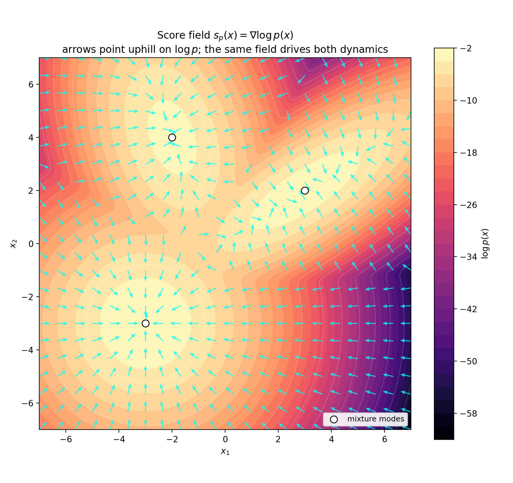
The score field $s_p(x)=\nabla\log p(x)$ of a three-component Gaussian mixture (colour = $\log p$, open circles = modes). Arrows point uphill toward the modes; the same field drives both dynamics below.
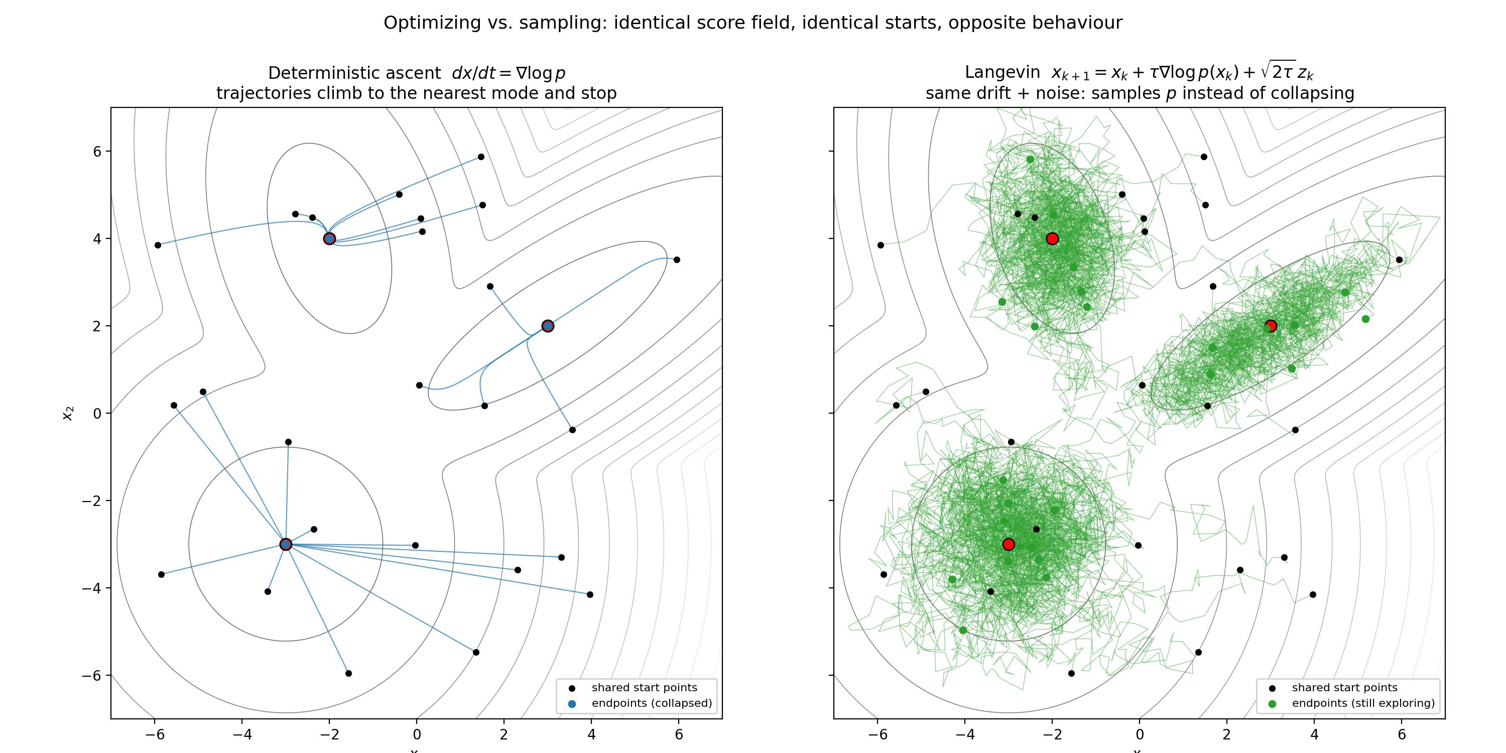
Twenty-five trajectories from the same shared start points (black). Left: deterministic ascent $dx/dt=\nabla\log p$ collapses each start to the nearest mode and stops. Right: the Langevin update $x_{k+1}=x_k+\tau\nabla\log p(x_k)+\sqrt{2\tau}\,z_k$ keeps wandering and spreads across all three modes — sampling $p$ instead of optimizing it. (With well-separated modes, recovering the relative masses can require many steps, the slow-mixing issue analysed in [SE19], §3.2.2.)
Python source (numpy + matplotlib; scipy optional)
"""
Langevin dynamics vs. deterministic score ascent on a 2D Gaussian mixture.

Companion to entries/mathematics/langevin-dynamics.html.
Run: python3 01_langevin_score_field.py   (writes into ./figures/)

The SCORE of a density p is the vector field

        s_p(x) = grad_x log p(x),

i.e. the direction of steepest increase of the log-density. Two dynamics use
the same score but behave very differently:

  - Deterministic score ascent  dx/dt = grad log p(x)
        a gradient flow on log p; every trajectory climbs to the nearest mode
        and STOPS there. It optimizes.

  - Langevin (overdamped) diffusion  dX_t = grad log p(X_t) dt + sqrt(2) dW_t
        the same drift plus Brownian noise. Its invariant law is p itself, so
        trajectories do not collapse: they keep wandering and, over time, visit
        each mode in proportion to its probability mass. It samples.

This script makes that contrast visible.
"""

import numpy as np
import matplotlib

matplotlib.use("Agg")  # headless: write PNGs without a display
import matplotlib.pyplot as plt
from pathlib import Path

# scipy is optional; fall back to a numerically stable manual logsumexp.
try:
    from scipy.special import logsumexp as _logsumexp

    def logsumexp(a, axis=None, keepdims=False):
        return _logsumexp(a, axis=axis, keepdims=keepdims)

except Exception:  # scipy unavailable

    def logsumexp(a, axis=None, keepdims=False):
        """Stable log-sum-exp: log sum_i exp(a_i), shifting by the max."""
        a = np.asarray(a)
        a_max = np.max(a, axis=axis, keepdims=True)
        a_max = np.where(np.isfinite(a_max), a_max, 0.0)
        out = np.log(np.sum(np.exp(a - a_max), axis=axis, keepdims=True)) + a_max
        if keepdims:
            return out
        return np.squeeze(out, axis=axis) if axis is not None else out.reshape(())


# --------------------------------------------------------------------------
# Target density: a mixture of three Gaussians with distinct weights/covariances
# --------------------------------------------------------------------------
WEIGHTS = np.array([0.5, 0.3, 0.2])          # mixing weights, sum to 1
MEANS = np.array([[-3.0, -3.0],              # mode 1
                  [3.0, 2.0],                # mode 2
                  [-2.0, 4.0]])              # mode 3
COVS = np.array([[[1.0, 0.0], [0.0, 1.0]],          # round
                 [[1.6, 0.9], [0.9, 0.8]],          # tilted, anisotropic
                 [[0.6, -0.3], [-0.3, 1.4]]])       # tilted the other way

# Precompute per-component constants.
_INV_COVS = np.linalg.inv(COVS)                              # (K,2,2)
_LOG_NORM = -0.5 * (2 * np.log(2 * np.pi) + np.log(np.linalg.det(COVS)))  # (K,)
_LOG_W = np.log(WEIGHTS)                                     # (K,)


def _component_logpdf(X):
    """Per-component log N(x; mu_k, Sigma_k).  X:(N,2) -> (N,K)."""
    d = X[:, None, :] - MEANS[None, :, :]                   # (N,K,2)
    # quadratic form d^T Sigma^{-1} d via einsum
    q = np.einsum("nki,kij,nkj->nk", d, _INV_COVS, d)       # (N,K)
    return _LOG_NORM[None, :] - 0.5 * q                     # (N,K)


def log_p(X):
    """Exact log density log p(x) of the mixture.  X:(N,2) -> (N,)."""
    comp = _component_logpdf(X) + _LOG_W[None, :]           # (N,K)
    return logsumexp(comp, axis=1)


def score(X):
    """
    Exact score grad_x log p(x) for the mixture.  X:(N,2) -> (N,2).

    For p = sum_k w_k N_k, the score is a responsibility-weighted average of
    each component's score grad log N_k(x) = -Sigma_k^{-1} (x - mu_k):

        grad log p(x) = sum_k r_k(x) * [ -Sigma_k^{-1}(x - mu_k) ],
        r_k(x) = w_k N_k(x) / sum_j w_j N_j(x)   (the soft mode-assignment).
    """
    comp = _component_logpdf(X) + _LOG_W[None, :]           # (N,K)
    log_r = comp - logsumexp(comp, axis=1, keepdims=True)
    r = np.exp(log_r)                                        # (N,K) responsibilities
    d = X[:, None, :] - MEANS[None, :, :]                   # (N,K,2)
    comp_score = -np.einsum("kij,nkj->nki", _INV_COVS, d)   # (N,K,2)
    return np.einsum("nk,nki->ni", r, comp_score)           # (N,2)


# --------------------------------------------------------------------------
# Grid over [-7,7] x [-7,7]
# --------------------------------------------------------------------------
LO, HI = -7.0, 7.0
gx = np.linspace(LO, HI, 220)
gy = np.linspace(LO, HI, 220)
GX, GY = np.meshgrid(gx, gy)
GRID = np.column_stack([GX.ravel(), GY.ravel()])
LOGP = log_p(GRID).reshape(GX.shape)


# --------------------------------------------------------------------------
# Trajectory integrators
# --------------------------------------------------------------------------
def deterministic_paths(x0, n_steps=400, tau=0.05):
    """Euler steps of the gradient flow  x <- x + tau * grad log p(x)."""
    x = x0.copy()
    traj = [x.copy()]
    for _ in range(n_steps):
        x = x + tau * score(x)
        traj.append(x.copy())
    return np.array(traj)  # (n_steps+1, N, 2)


def langevin_paths(x0, n_steps=400, tau=0.05, rng=None):
    """
    Unadjusted Langevin: x <- x + tau * grad log p(x) + sqrt(2 tau) * z,  z ~ N(0,I).

    Why sqrt(tau)?  The noise discretizes Brownian motion dW_t. Over a step of
    size tau, the Brownian increment has variance tau (Var[W_{t+tau}-W_t]=tau),
    so its standard deviation scales as sqrt(tau) -- NOT tau. The drift is O(tau);
    the noise is O(sqrt(tau)) and therefore dominates as tau -> 0. That surviving
    noise is exactly what stops the iterate from freezing at a mode and instead
    makes it SAMPLE from p rather than merely optimize log p.
    """
    if rng is None:
        rng = np.random.default_rng(0)
    x = x0.copy()
    traj = [x.copy()]
    coeff = np.sqrt(2.0 * tau)
    for _ in range(n_steps):
        z = rng.standard_normal(x.shape)
        x = x + tau * score(x) + coeff * z
        traj.append(x.copy())
    return np.array(traj)  # (n_steps+1, N, 2)


# --------------------------------------------------------------------------
# Figure 1: log-density contours + score vector field
# --------------------------------------------------------------------------
def figure_score_field(out_path):
    fig, ax = plt.subplots(figsize=(8.5, 8.0))
    cs = ax.contourf(GX, GY, LOGP, levels=30, cmap="magma")
    ax.contour(GX, GY, LOGP, levels=12, colors="white", linewidths=0.4, alpha=0.5)

    # coarse quiver of the score field; normalize arrows to show direction
    qn = 22
    qx = np.linspace(LO, HI, qn)
    qy = np.linspace(LO, HI, qn)
    QX, QY = np.meshgrid(qx, qy)
    S = score(np.column_stack([QX.ravel(), QY.ravel()]))
    U = S[:, 0].reshape(QX.shape)
    V = S[:, 1].reshape(QX.shape)
    mag = np.hypot(U, V) + 1e-12
    ax.quiver(QX, QY, U / mag, V / mag, color="cyan", alpha=0.8,
              scale=34, width=0.0025, headwidth=4)
    ax.scatter(MEANS[:, 0], MEANS[:, 1], c="white", edgecolors="black",
               s=70, zorder=5, label="mixture modes")

    ax.set_xlim(LO, HI)
    ax.set_ylim(LO, HI)
    ax.set_aspect("equal")
    ax.set_xlabel("$x_1$")
    ax.set_ylabel("$x_2$")
    ax.set_title("Score field $s_p(x)=\\nabla\\log p(x)$\n"
                 "arrows point uphill on $\\log p$; the same field drives both dynamics")
    ax.legend(loc="lower right", framealpha=0.9, fontsize=9)
    fig.colorbar(cs, ax=ax, shrink=0.85, label="$\\log p(x)$")
    fig.tight_layout()
    fig.savefig(out_path, dpi=200)
    plt.close(fig)


# --------------------------------------------------------------------------
# Figure 2: deterministic ascent vs. Langevin sampling, shared starts
# --------------------------------------------------------------------------
def figure_compare(out_path, n_paths=25, n_steps=400, tau=0.05):
    rng = np.random.default_rng(7)
    # SAME initial points for both panels: spread broadly over the domain
    x0 = rng.uniform(LO + 1, HI - 1, size=(n_paths, 2))

    det = deterministic_paths(x0, n_steps=n_steps, tau=tau)
    lan = langevin_paths(x0, n_steps=n_steps, tau=tau,
                         rng=np.random.default_rng(11))

    fig, axes = plt.subplots(1, 2, figsize=(15.0, 7.5), sharex=True, sharey=True)
    for ax in axes:
        ax.contour(GX, GY, LOGP, levels=12, cmap="Greys",
                   linewidths=0.6, alpha=0.6)
        ax.scatter(MEANS[:, 0], MEANS[:, 1], c="red", edgecolors="black",
                   s=70, zorder=6)
        ax.scatter(x0[:, 0], x0[:, 1], c="black", s=14, zorder=5,
                   label="shared start points")
        ax.set_xlim(LO, HI)
        ax.set_ylim(LO, HI)
        ax.set_aspect("equal")
        ax.set_xlabel("$x_1$")

    # left: deterministic -> collapse to modes
    for i in range(n_paths):
        axes[0].plot(det[:, i, 0], det[:, i, 1], color="tab:blue",
                     lw=0.8, alpha=0.7)
    axes[0].scatter(det[-1, :, 0], det[-1, :, 1], c="tab:blue",
                    s=22, zorder=7, label="endpoints (collapsed)")
    axes[0].set_ylabel("$x_2$")
    axes[0].set_title("Deterministic ascent  $dx/dt=\\nabla\\log p$\n"
                      "trajectories climb to the nearest mode and stop")
    axes[0].legend(loc="lower right", framealpha=0.9, fontsize=8)

    # right: Langevin -> keeps exploring, spreads across mass
    for i in range(n_paths):
        axes[1].plot(lan[:, i, 0], lan[:, i, 1], color="tab:green",
                     lw=0.5, alpha=0.5)
    axes[1].scatter(lan[-1, :, 0], lan[-1, :, 1], c="tab:green",
                    s=22, zorder=7, label="endpoints (still exploring)")
    axes[1].set_title("Langevin  $x_{k+1}=x_k+\\tau\\nabla\\log p(x_k)+\\sqrt{2\\tau}\\,z_k$\n"
                      "same drift + noise: samples $p$ instead of collapsing")
    axes[1].legend(loc="lower right", framealpha=0.9, fontsize=8)

    fig.suptitle("Optimizing vs. sampling: identical score field, "
                 "identical starts, opposite behaviour", fontsize=13)
    fig.tight_layout(rect=(0, 0, 1, 0.96))
    fig.savefig(out_path, dpi=200)
    plt.close(fig)


def main():
    out_dir = Path(__file__).parent / "figures"
    out_dir.mkdir(exist_ok=True)
    f1 = out_dir / "01_score_field.png"
    f2 = out_dir / "02_deterministic_vs_langevin.png"

    figure_score_field(f1)
    figure_compare(f2)

    print("Saved:")
    print(f"  {f1}")
    print(f"  {f2}")


if __name__ == "__main__":
    main()
Source for the discrete update and the Gaussian-mixture diagnostic: [SE19] = Yang Song & Stefano Ermon, “Generative Modeling by Estimating Gradients of the Data Distribution,” NeurIPS 2019 (arXiv:1907.05600) — Eq. 4 is the Langevin sampling step used here; §3.2.2 and Fig. 2 use a mixture of Gaussians to illustrate the score field and the slow mixing of Langevin dynamics between well-separated modes. The continuous SDEs (L1)/(L2) and their shared invariant law are standard overdamped-Langevin facts. — the same space of measures, read historically: Concepts as measures; and a transport bound that diagnoses a learned sampler's mode weights, a mixture-coupling upper bound for $W_2^2$.
Hierarchical reinforcement learning: options and SMDPs
A short companion note, written toward the AC conjecture: why temporally extended decisions in hierarchical RL are naturally modeled as a semi-Markov decision process rather than a one-step Markov one.
§1. The formalization
The convenient mathematical model for temporally extended decisions in hierarchical RL is a semi-Markov decision process (SMDP), whose uncontrolled dynamics reduce to a semi-Markov process (SMP). The key feature is that the time between decisions is itself random.
Remark (why semi-Markov). An option (macro-action) induces a random
execution duration. If decisions are made only at option-termination times, the resulting
decision process is naturally semi-Markov rather than one-step Markov in physical time. This
is the reason SMDPs are the standard formalism for options.
This is a stub I expect to grow: the next step is to state the SMP definition precisely and connect the option framework to the search structure used in the RL-algorithms note.
Function-space consolidation
The previous entry protected parameters. Several recent methods instead protect the function the generator implements, and in replay-free personalization the dominant family is no longer full finetuning but parameter-efficient finetuning (PEFT). This entry covers function-space distillation, the PEFT zoo, concept-structure-aware customization, and the separate use of diffusion models as rehearsal machinery for other learners.
§1. Function-space distillation
Rather than anchoring weights, match teacher and student in function space. In continual personalization via diffusion classifier scores this is a double-distillation strategy: keep a Fisher-like parameter penalty and preserve old concepts by matching diffusion classifier scores on selected concepts. Schematically, $$ \c{L}^{\mathrm{func}}_t(\theta) = \EE_{x,\c{S}}\sqbr{D\smbr{S_\theta(\cdot\mid x,\c{S}),\,S_{\bar\theta_{t-1}}(\cdot\mid x,\c{S})}}, $$ where $S_\theta$ is a score-based class posterior over a concept subset $\c{S}$ and $D$ is a discrepancy (KL or squared error). Conceptually this is closer to model consolidation than to pure replay.1
§2. PEFT: adapters, LoRA, masks, neurons
The generic idea: freeze the pretrained backbone, train a small structured set.
- LoRA. Write a weight matrix as $W=W_0+B_t A_t$, with $W_0$ frozen and $A_t,B_t$ low-rank trainable factors for task $t$. Interference is confined to a small subspace and task-specific residuals are cheap to store.2
- C-LoRA. Continual customization with low-rank updates in cross-attention
plus a self-regularization term discouraging new LoRA weights from overwriting used
support:
$$ \c{L}^{\mathrm{C\text{-}LoRA}}_t = \c{L}^{\mathrm{new}}_t + \lambda\,R_{\mathrm{self}}(A_t,B_t;\crbr{A_s,B_s}_{s
- STAMINA. Stack-and-mask incremental adapters: low-rank adapters paired with learnable hard attention masks (small MLPs), foldable back into the model after training to avoid inference-time growth. Designed to scale to long concept sequences without replay.3
- CNS (Concept Neuron Selection). Identify neurons related to the incoming concept and update only those, preserving earlier zero-shot ability — not all backbone parameters need to stay plastic.4
§3. Concept-structure-aware customization
A second line exploits the structure of the concept space itself.
- CIDM / CIFC. Formalizes Concept-Incremental Flexible Customization across objects, styles, and edits. Its loss adds a concept-consolidation term for task-specific and task-shared knowledge plus elastic weight aggregation: $$ \c{L}^{\mathrm{CIDM}}_t = \c{L}^{\mathrm{new}}_t + \lambda_{\mathrm{sp}}\c{L}_{\mathrm{TSP}} + \lambda_{\mathrm{sh}}\c{L}_{\mathrm{TSH}}, $$ with inference-time aggregation of historical low-rank weights. The goal is to avoid both forgetting and concept neglect — failing to realize all requested concepts in a joint prompt.5
- ConceptGuard. Targets both concept forgetting and concept confusion via shift embeddings, concept-binding prompts, memory-preservation regularization, and a concept priority queue — especially relevant when old and new concepts are semantically confusable.6
§4. Diffusion as rehearsal machinery
In parallel, diffusion models are used as memory systems for other continual learners.
- Image-level replay. DDGR uses a diffusion generator plus classifier-derived guidance for class-incremental rehearsal; SDDR uses Stable Diffusion for class-matched synthetic images for both replay and distillation; DiffusePast extends this to class-incremental semantic segmentation, SDDGR to object detection.7
- The synthetic–real gap. Synthetic replay does not match the real training distribution. DiffClass reframes exemplar-free CIL as multi-domain adaptation — diffusion generation plus multi-distribution matching, selective augmentation, and domain-adversarial training — so the model discriminates “class vs. class” rather than “real vs. synthetic.”8
- Feature replay. DiffFR trains a diffusion model on features, not pixels: with a fixed extractor $\phi(x)$, sample $\hat h\sim p_\psi(h\mid y)$, $h=\phi(x)$, and update a linear classifier — reducing the replay problem's complexity, strong in non-exemplar CIL.9
- Joint models. JDCL jointly parameterizes classifier and diffusion replay model in one network with distillation, reducing redundancy between representation learning and replay generation.10
§5. What currently seems to work
- Direct continual training of generators: replay is the strongest generic baseline, but it is diffusion-specific (timestep effects; endpoint-only protection is insufficient). Generative distillation and diffusion-aware Fisher penalties are natural upgrades.11
- Replay-free personalization: PEFT and structured consolidation dominate — from early LoRA regularization (C-LoRA) toward richer consolidation (diffusion classifier scores), masked adapters (STAMINA), and concept-structured methods (CIDM, ConceptGuard, CNS).
- Foundation-model post-training: no universally best method; retention of the prior, downstream adaptation, forgetting, and cross-task composition pull in different directions.
- Diffusion-assisted downstream CL: the bottleneck is often the synthetic–real gap, so methods that attack it directly are strongest.
Bottom line. Diffusion models did not change the stability–plasticity
dilemma; they changed where it lives. One must now preserve a denoising trajectory,
a conditioning interface, a pretrained generative prior, and often a compositional prompt
semantics — all at once. Continual learning for diffusion is not the old taxonomy with a new
backbone, but a genuinely richer sequential-learning problem.
1 Jha et al., “Diffusion classifier scores for continual personalization,” ICLR 2025. 2 Smith et al. (C-LoRA), arXiv:2304.06027. 3 Smith et al. (STAMINA), arXiv:2311.18763. 4 Liao et al. (CNS / continual personalization), arXiv:2510.02296. 5 Dong et al. (CIDM/CIFC), arXiv:2410.17594. 6 Guo & Jin (ConceptGuard), arXiv:2503.10358. 7 Gao & Liu (DDGR), ICML 2023; Jodelet et al. (SDDR), arXiv:2306.17560; Chen et al. (DiffusePast), arXiv:2308.01127; Kim et al. (SDDGR), arXiv:2402.17323. 8 Meng et al. (DiffClass), arXiv:2403.05016. 9 Zhang et al. (DiffFR), arXiv:2408.02983. 10 Skierś & Deja (JDCL), arXiv:2411.08224. 11 Zając et al., arXiv:2303.15342; Masip et al., arXiv:2311.14028; Wang et al., arXiv:2509.23593; Huang et al., arXiv:2505.16875. — appendix: the DDPM machinery underlying all of this.
Forgetting and elastic weight consolidation
The central failure mode of continual learning is forgetting: after training on new data, performance on previously learned tasks deteriorates. The strongest form, catastrophic forgetting, is when sequential gradient updates for a new task substantially overwrite parameters important for earlier tasks. The right reading is not “change in parameters” but loss of previously acquired competence under sequential training.1
§1. Three mitigation families
- Regularization-based. Estimate which parameters matter for old tasks and penalize changes to them. EWC, synaptic intelligence (SI), memory-aware synapses (MAS).
- Architectural / parameter-isolation. Reduce interference by separating, freezing, or routing parameters: classical modular subnetworks, and modern PEFT (adapters, LoRA) that freeze the base model and train a small set of extra parameters.
- Replay / rehearsal. Revisit past data, either stored in an episodic memory or synthesized by a generative model.2
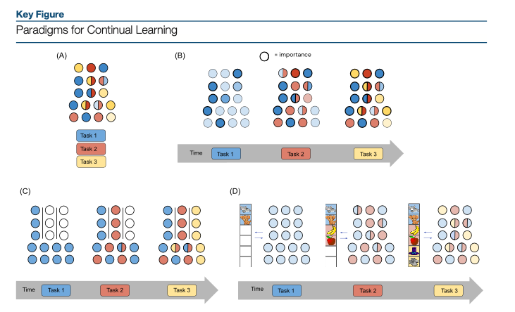
Schematic taxonomy: regularization protects important parameters; architectural methods isolate or freeze them; replay revisits past experience through stored or generated samples.
This entry develops the regularization family; replay is the next one, and parameter isolation reappears in function-space consolidation.
§2. Elastic weight consolidation
Suppose a model $\theta\in\RR^d$ is first trained on task $A$, giving $\theta_A^\ast\in\arg\min_\theta \c{L}_A(\theta)$. When task $B$ arrives, naive fine-tuning minimizes only $\c{L}_B(\theta)$ and may move $\theta$ far from values needed for $A$. EWC starts from the Bayesian identity $$ p(\theta\mid\c{D}_A,\c{D}_B) \propto p(\c{D}_B\mid\theta)\,p(\theta\mid\c{D}_A), $$ assuming $p(\c{D}_B\mid\theta,\c{D}_A)=p(\c{D}_B\mid\theta)$. So learning $B$ after $A$ means maximizing the new-task likelihood while retaining the posterior from $A$.
EWC approximates the old posterior near $\theta_A^\ast$ by a Gaussian — a second-order expansion of the negative log-posterior: $$ -\log p(\theta\mid\c{D}_A) \approx \text{const} + \frac12\sum_{i=1}^d F_{A,i}\,(\theta_i-\theta_{A,i}^\ast)^2, $$ where $\theta_i$ is the $i$-th parameter component and $F_{A,i}$ is the $i$-th diagonal entry of the Fisher information $$ F_{A,ij} := \EE_{(x,y)\sim\c{D}_A}\sqbr{\partial_{\theta_i}\log p(y\mid x,\theta_A^\ast)\,\partial_{\theta_j}\log p(y\mid x,\theta_A^\ast)} $$ evaluated at $\theta_A^\ast$, so $F_{A,i}=\EE_{(x,y)\sim\c{D}_A}\sqbr{(\partial_{\theta_i}\log p(y\mid x;\theta_A^\ast))^2}$. Dropping constants gives the EWC objective:
$$ \c{L}_{\mathrm{EWC}}(\theta) = \c{L}_B(\theta) + \frac{\lambda}{2}\sum_{i=1}^d F_{A,i}\,(\theta_i-\theta_{A,i}^\ast)^2. $$
Here $\lambda>0$ controls the stability–plasticity trade-off: large $\lambda$ protects old knowledge but may starve adaptation to $B$. If $F_{A,i}$ is large, task $A$ was very sensitive to $\theta_i$, so moving it is expensive; if small, that coordinate may move freely. EWC thus implements an anisotropic quadratic trust region around $\theta_A^\ast$.
§3. A two-parameter example
Let $\theta=(w_1,w_2)$, with task-$A$ optimum $\theta_A^\ast=(2,0)$ and diagonal Fisher $F_A=(100,1)$ — $w_1$ is judged very important, $w_2$ much less. Let task $B$ have loss $\c{L}_B(w_1,w_2)=(w_1-1)^2+(w_2-3)^2$, whose unregularized optimum $(1,3)$ moves far in both coordinates. With EWC and $\lambda=1$, $$ \c{L}_{\mathrm{EWC}} = (w_1-1)^2+(w_2-3)^2 + \tfrac12\sqbr{100(w_1-2)^2 + (w_2-0)^2}. $$ Setting derivatives to zero, $2(w_1-1)+100(w_1-2)=0$ and $2(w_2-3)+w_2=0$, so $$ w_1=\tfrac{202}{102}\approx 1.98, \qquad w_2=2. $$ EWC allows substantial movement in the weakly constrained direction $w_2$ but keeps $w_1$ close to the value $A$ requires — exactly the intended behavior.
§4. Status of the objective
The penalty is an approximation to sequential Bayesian updating. Since $p(\theta\mid\c{D}_A)$ is intractable in deep networks, EWC takes a Laplace approximation around $\theta_A^\ast$, $$ -\log p(\theta\mid\c{D}_A) \approx \text{const} + \tfrac12(\theta-\theta_A^\ast)^\top H_A(\theta-\theta_A^\ast), $$ approximates the Hessian $H_A$ by the Fisher $F_A$, and discards off-diagonal entries: $(\theta-\theta_A^\ast)^\top F_A(\theta-\theta_A^\ast)\approx\sum_i F_{A,i}(\theta_i-\theta_{A,i}^\ast)^2$. A tunable scalar $\lambda$ then sets the strength of this old-task penalty.
So the usual diagonal EWC objective is not exact Bayes but a
Laplace–Fisher–diagonal approximation with a tunable regularization scale. In
practice one uses the diagonal empirical Fisher estimated from task-$A$ gradients:
cheap, but it ignores parameter correlations and is only local near $\theta_A^\ast$. The
diffusion-specific successor — a rank-1 Fisher — is developed
later.
1 French, “Catastrophic forgetting in connectionist networks,” TiCS 1999; Kirkpatrick et al., “Overcoming catastrophic forgetting in neural networks,” PNAS 114(13) 2017. 2 van de Ven & Tolias, arXiv:1904.07734; Robins, “Catastrophic forgetting, rehearsal and pseudorehearsal,” Connection Science 1995. — next: replay and iCaRL; the Fisher returns for diffusion in weight regularization.
Weight regularization and diffusion consolidation
Regularization methods stay relevant for diffusion models, but they behave differently than in discriminative networks. The interesting recent twist is that the empirical Fisher of a diffusion model is often approximately rank-1 — most curvature concentrates in a single parameter-space direction — which yields an EWC nearly as cheap as the diagonal version but capturing a dominant shared direction. This entry builds up to that.
§1. The two baselines
L2 anchoring penalizes deviation from old parameters, $\Omega_t^{L2}(\theta)=\tfrac12\norm{\theta-\theta_{t-1}^\star}_2^2$, and appears as a baseline in both direct continual DDPM training and later post-training benchmarks.1 EWC-style consolidation uses a Fisher-weighted quadratic penalty, $$ \Omega_t^{\mathrm{EWC}}(\theta) = \frac12\sum_{i=1}^d F_i^{(\le t-1)}(\theta_i-\theta_{t-1,i}^\star)^2. $$ In replay-free personalization, the diffusion-classifier-score work argues that the standard C-LoRA self-regularization loses plasticity over long sequences, and instead builds Fisher estimates from diffusion classifier scores, combining parameter-space consolidation with a complementary function-space term.2
§2. Fisher in EWC, recalled
EWC starts from sequential Bayesian updating (the discriminative derivation is in forgetting and EWC). With task datasets $D_1,\dots,D_T$, $$ p(\theta\mid D_{1:T}) \propto p(D_T\mid\theta)\,p(\theta\mid D_{1:T-1}), $$ and a Laplace approximation of the previous-task posterior around $\theta_{T-1}^\star$ gives $$ -\log p(\theta\mid D_{1:T-1}) \approx \tfrac12(\theta-\theta_{T-1}^\star)^\top F^{(T-1)}(\theta-\theta_{T-1}^\star), $$ hence $$ L_{\mathrm{EWC}}(\theta) = L_T(\theta) + \frac{\lambda}{2}(\theta-\theta_{T-1}^\star)^\top F^{(T-1)}(\theta-\theta_{T-1}^\star). $$ Directions of larger old-task Fisher curvature are penalized more, because moving along them changes the previous model most. The Fisher is a local importance matrix.3
§3. How a Fisher enters diffusion training
DDPM is not optimized by differentiating a tractable $\log p_\theta(x_0)$. One trains the denoiser with the per-sample loss $$ L_{\mathrm{simple}}(\theta;x_t,t,\epsilon)=\tfrac12\norm{\epsilon-\epsilon_\theta(x_t,t)}_2^2,\qquad x_t=\sqrt{\bar\alpha_t}\,x_0+\sqrt{1-\bar\alpha_t}\,\epsilon, $$ which is denoising score matching since $\epsilon_\theta(x_t,t)=-\sqrt{1-\bar\alpha_t}\,s_\theta(x_t,t)$ and $\EE[\epsilon\mid x_t]=-\sqrt{1-\bar\alpha_t}\,s_t^\star(x_t)$. To get a clean Fisher, introduce the auxiliary Gaussian observation model $r_\theta(\epsilon\mid x_t,t)=\c{N}(\epsilon;\epsilon_\theta(x_t,t),I)$, for which $-\log r_\theta(\epsilon\mid x_t,t)=\tfrac12\norm{\epsilon-\epsilon_\theta(x_t,t)}_2^2$ up to a constant — exactly the DDPM loss. Then the gradient outer-product matrix $$ F_{\mathrm{aux}}(\theta) = \EE\sqbr{\nabla_\theta L_{\mathrm{simple}}(\theta)\,\nabla_\theta L_{\mathrm{simple}}(\theta)^\top} $$ is the classical Fisher of that Gaussian model. In score-matching form, with $g(x_t;\theta):=\nabla_\theta L_{\mathrm{DSM}}(\theta;x_t)$, the per-timestep empirical Fisher is $F_t(\theta):=\EE_{x_t\sim q_t}\sqbr{g(x_t;\theta)g(x_t;\theta)^\top}$ — a curvature matrix for the diffusion surrogate, estimated through gradient outer products along the sampling process.4
§4. What rank-1 means, exactly
Let $F\in\RR^{m\times m}$ be symmetric PSD. By the spectral theorem $F=\sum_{i=1}^m\lambda_i u_i u_i^\top$ with $\lambda_1\ge\dots\ge\lambda_m\ge0$ and orthonormal $\crbr{u_i}$. $F$ is exactly rank-1 iff $\lambda_1>0$ and $\lambda_2=\dots=\lambda_m=0$, i.e. $F=\lambda_1 u_1 u_1^\top$. Then for a perturbation $\delta$, $$ \delta^\top F\delta = \lambda_1(u_1^\top\delta)^2, $$ so only the component of $\delta$ along $u_1$ is penalized; everything orthogonal to $u_1$ is in the nullspace and costs nothing.
In practice one expects only approximate rank-1: $\lambda_1\gg\lambda_2,\dots,\lambda_m$,
i.e. $F\approx\lambda_1 u_1 u_1^\top$. Geometrically, most curvature concentrates along one
dominant direction. Wang et al. observe diffusion gradients in low-SNR regimes become
strongly collinear, so the empirical Fisher is approximately rank-1. The resulting
rank-1 EWC is nearly as cheap as diagonal EWC but captures a dominant shared
curvature direction; combined with replay it improved average FID and reduced forgetting
relative to replay-only and diagonal-EWC baselines on class-incremental generation.4
1 Zając et al., arXiv:2303.15342; Huang et al. (T2I-ConBench), arXiv:2505.16875. 2 Jha et al., “Diffusion classifier scores for continual personalization,” ICLR 2025. 3 Kirkpatrick et al., PNAS 2017. 4 Wang et al., “Avoid catastrophic forgetting with rank-1 Fisher from diffusion models,” arXiv:2509.23593; Ho, Jain & Abbeel, arXiv:2006.11239. — the complementary function-space methods are next.
Problem statements for CL with diffusion models
Diffusion models change the formal object of continual learning. In the discriminative setting one sequentially updates a predictor $f_\theta:\c{X}\to\c{Y}$. A diffusion model instead learns a time-indexed denoising field (equivalently a score field), so the thing being protected is a whole reverse process and a conditioning interface, not a decision boundary. This entry sets up the object and recasts the three scenarios; the underlying DDPM machinery is in the appendix.
§1. The learned object
In the DDPM parameterization, start from clean data $x_0\in\c{X}$, sample a diffusion timestep $u\in\crbr{1,\dots,U}$ and noise $\epsilon\sim\c{N}(0,I)$, form $x_u=\alpha_u x_0+\sigma_u\epsilon$, and train a network $\epsilon_\theta(x_u,u,c)$ — conditioned on side information $c$ — to predict the injected noise: $$ \ell_{\mathrm{diff}}(x_0,c;\theta) = \EE_{u,\epsilon}\sqbr{w_u\,\norm{\epsilon-\epsilon_\theta(\alpha_u x_0+\sigma_u\epsilon,u,c)}_2^2}. $$ In the score-SDE view the same object is a score network $s_\theta(x_u,u,c)\approx\nabla_x\log p_u(x\mid c)$ driving a reverse-time SDE; latent diffusion applies the same formalism in a learned latent $z_0=E(x_0)$.1
Definition (generic continual diffusion learning). A continual diffusion
problem consists of a state space $\c{X}$ (pixels, latents, clips, features); conditioning
spaces $\c{C}_1,\dots,\c{C}_T$; datasets $\c{D}_t\subseteq\c{X}\times\c{C}_t$,
$\c{D}_t\sim P_t$; and an update rule
$$ \theta_t = U_t(\theta_{t-1},\c{D}_t,\c{M}_{t-1}), $$
where $\c{M}_{t-1}$ is any retained memory (real or synthetic samples, adapters, Fisher
summaries, teacher snapshots). The learner must adapt $p_{\theta_t}(x\mid c)$ to $P_t$ while
preserving competence on $\crbr{P_s(\cdot\mid c):s
§2. Diffusion analogues of the three scenarios
The Task/Domain/Class split from the discriminative entry transfers cleanly.
- Task-conditioned generation. Task identity $\tau$ is available at sampling time: learn $p_\theta(x\mid c,\tau)$, $c\in\c{C}_\tau$. Most permissive — task embeddings, separate heads, task adapters, routing all allowed. Early continual-DDPM studies condition a single model on a task identifier as tasks arrive.2
- Domain-incremental generation. Task identity is not available, but the conditioning interface is shared: learn one $p_\theta(x\mid c)$, $c\in\c{C}$, while the conditional law drifts, $P_t(X\mid c)\neq P_s(X\mid c)$. The challenge is preserving sample quality under drift, not enlarging the conditioning alphabet — e.g. continual domain enhancement for text-to-image models.3
- Class- / concept-incremental generation. The conditioning alphabet expands, $\c{C}^{(\le t)}:=\bigcup_{s\le t}\c{C}_s$, and after task $t$ the model must support $p_{\theta_t}(x\mid c)$ for $c\in\c{C}^{(\le t)}$ with no oracle for the concept's origin task. The natural formalization for continual personalization and concept addition. The hard part is preserving the semantics of the conditioning interface: an old token or label must still denote the same concept after later updates.4
§3. Three regimes worth separating
The literature splits into practically distinct regimes; three matter most here.
(i) Continual generative modeling of changing image distributions. For
distributions $P_1,\dots,P_T$ on $\c{X}\times\c{Y}$, produce $\theta_1,\dots,\theta_T$ with
$p_{\theta_t}(x\mid y)$ modeling $P_t(x\mid y)$ while retaining $P_s$, $s
(ii) Continual post-training of pretrained text-to-image models. Start from a pretrained $p_{\theta_0}(x\mid\pi)$ on a large base $P_{\mathrm{base}}$; the stream is small task datasets $\c{D}_t=\crbr{(x_i,\pi_i)}_{i=1}^{n_t}$, $n_t\ll|P_{\mathrm{base}}|$, with $\theta_t=\c{A}_t(\theta_{t-1},\c{D}_t,M_{t-1})$. The goal is to fit $\c{D}_t$ while retaining (a) pretrained generality on $P_{\mathrm{base}}$, (b) earlier downstream tasks, (c) zero-shot compositionality. An abstract objective: $$ \min_\theta\ \c{L}_{\mathrm{cur}}(\theta;\c{D}_t) + \lambda_{\mathrm{old}}\c{R}_{\mathrm{old}}(\theta;\theta_{t-1},M_{t-1}) + \lambda_{\mathrm{base}}\c{R}_{\mathrm{base}}(\theta;\theta_0). $$ T2I-ConBench makes the regime explicit, separating item customization and domain enhancement, and four evaluation axes — retained base capability, current-task adaptation, backward transfer, and cross-task compositionality.3
(iii) Replay-free continual personalization. A special case of (ii): task
$t$ introduces a new concept $c_t$ from a few examples
$\c{D}_t=\crbr{(x_i,\pi_i(\omega_t))}$, where $\omega_t$ is the inference-time handle (a
learned token, a LoRA state, a neuron mask), with cumulative vocabulary
$\Omega_{\le t}=\crbr{\omega_1,\dots,\omega_t}$. No raw samples from
$\bigcup_{s
1 Ho, Jain & Abbeel, “Denoising diffusion probabilistic models,” arXiv:2006.11239; Song et al., “Score-based generative modeling through SDEs,” ICLR 2021.
2 Zając et al., “Exploring continual learning of diffusion models,” arXiv:2303.15342.
3 Huang et al., “T2I-ConBench,” arXiv:2505.16875.
4 Smith et al. (C-LoRA) arXiv:2304.06027; Dong et al. arXiv:2410.17594; Jha et al. (diffusion classifier scores) ICLR 2025.
5 Masip et al., “Continual learning of diffusion models with generative distillation,” arXiv:2311.14028.
— next: a controlled synthetic family; then metrics and algorithms.
In this regime forgetting is not the only failure mode: concept confusion can crater
compositional accuracy $C_t$ even when single-concept identity scores stay fine. Methods:
C-LoRA, STAMINA, diffusion-classifier-score regularization, CIDM/CIFC, ConceptGuard, CNS
— all in function-space consolidation.4
Metrics for CL with diffusion models
In diffusion continual learning the entry $(t,k)$ of the performance matrix is typically not a scalar but a vector. Visually plausible samples, correct prompt following, old-task retention, and compositional reuse can each fail independently, so a single number hides exactly the trade-off one is trying to study. This entry organizes the metrics into four families and shows why they disagree.
§1. A vector-valued performance matrix
Fix tasks $T_1,\dots,T_K$. For task $k$ let $\c{C}_k$ be the evaluation condition space, $\nu_k$ an evaluation distribution on $\c{C}_k$, and $P_k^{\mathrm{test}}$ the target image distribution. After training through task $t$ the conditional generator induces the task-marginal $$ P^{(k)}_{\theta_t}(A) := \int_{\c{C}_k} p_{\theta_t}(A\mid c)\,d\nu_k(c), \qquad A\subseteq\c{X}, $$ and for any metric $j$ we write $a_{t,k}^{(j)}:=\c{M}_k^{(j)}(\theta_t)$ — agnostic about whether $\c{M}_k^{(j)}$ is a distributional discrepancy, an alignment score, a forgetting score, or a compositional score.1
To aggregate, orient every metric so larger is better. With $s_j=+1$ for higher-better and $-1$ for lower-better, set $q_{t,k}^{(j)}:=s_j\,a_{t,k}^{(j)}$. Then the classical summaries carry over: $$ \mathrm{ACC}_t^{(j)}=\frac1t\sum_{k=1}^t q_{t,k}^{(j)},\qquad \mathrm{BWT}_t^{(j)}=\frac1{t-1}\sum_{k=1}^{t-1}\smbr{q_{t,k}^{(j)}-q_{k,k}^{(j)}}, $$ $$ \mathrm{FM}_t^{(j)}=\frac1{t-1}\sum_{k=1}^{t-1}\smbr{\max_{k\le\ell\le t-1}q_{\ell,k}^{(j)}-q_{t,k}^{(j)}}. $$
Metrics genuinely disagree. Suppose task 2 has FID $18.0$ right after
learning it, but $27.0$ after task 5. Since FID is lower-better, $q_{2,2}=-18.0$,
$q_{5,2}=-27.0$, so task 2's BWT contribution is $-9.0$ — clearly negative. If CLIP image
alignment on the same task rises $0.71\to0.76$, its BWT contribution is $+0.05$. The
same run can improve concept alignment while degrading distributional fidelity.
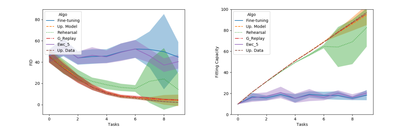
The same continual run, read through two different metrics over a task sequence — the curves do not have to move together.
§2. Distributional fidelity
A distributional metric compares the target $P_k^{\mathrm{test}}$ with the generated $P_{\theta_t}^{(k)}$ through a fixed feature map $\psi$ (Inception, CLIP image encoder, a video backbone): $$ d_{t,k}^{\mathrm{dist}} = \mathsf D\smbr{\psi_\#P_k^{\mathrm{test}},\,\psi_\#P_{\theta_t}^{(k)}}, $$ where $\psi_\#$ is pushforward. One is almost never comparing raw image distributions, but their images under $\psi$.2 The most common case is FID, $$ \mathrm{FID}_{t,k}=\|\mu_r-\mu_g\|_2^2+\operatorname{Tr}\!\smbr{\Sigma_r+\Sigma_g-2(\Sigma_r^{1/2}\Sigma_g\Sigma_r^{1/2})^{1/2}}. $$ Toy check: $\mu_r=(0,0)$, $\mu_g=(1,2)$, $\Sigma_r=I_2$, $\Sigma_g=\mathrm{diag}(4,1)$ give mean term $1^2+2^2=5$ and covariance term $1$, so $\mathrm{FID}=6$.
A more general family is maximum mean discrepancy: for a PD kernel $\kappa$, $$ \mathrm{MMD}_\kappa^2(P,Q)=\EE\,\kappa(X,X')+\EE\,\kappa(Y,Y')-2\EE\,\kappa(X,Y),\quad X,X'\sim P,\ Y,Y'\sim Q. $$ Kernel Inception Distance (KID) is an unbiased empirical MMD with a polynomial kernel on Inception features. Replacing those by CLIP image features and averaging across seen concepts gives an average MMD, $$ \mathrm{AMMD}_t=\frac1t\sum_{k=1}^t\mathrm{MMD}_\kappa\smbr{\phi_{\mathrm{img}}(X_k^{\mathrm{ref}}),\,\phi_{\mathrm{img}}(\hat X_{t,k})}, $$ natural for personalization, where the question is not “realistic?” but “still the same concept distribution?”3
Likelihood-style metrics are a different regime. If the model is a normalized density on a fixed $d$-dim image space, the bits-per-dimension score is $\mathrm{BPD}(x)=-\tfrac1{d\log 2}\log p_{\theta_t}(x)$ — meaningful for pixel-space DDPMs, usually not the right quantity for latent/adapter T2I post-training. Video reports Fréchet Video Distance (FVD) on spatiotemporal features.4
Remark (one scalar is not enough). Zając et al. show BPD can stay nearly
stable while old-task generation quality collapses. The explanation is timestep-wise: early
diffusion steps dominate the likelihood and stay intact, while later steps — crucial for
visible synthesis but minor for BPD — forget badly. A model can look fine under BPD and fail
under FID and inspection. BPD is at best a partial diagnostic.1
§3. Condition faithfulness
A latent T2I model is: a text encoder $\phi$ ($h=\phi(\pi)$); a VAE pair $(E,D)$ with $z_0=E(x)$, $x\approx D(z_0)$; and a denoiser $\epsilon_\theta(z_t,t,h)$ with cross-attention to tokens, trained on $z_t=\sqrt{\bar\alpha_t}\,z_0+\sqrt{1-\bar\alpha_t}\,\varepsilon$ to predict $\varepsilon$. In continual personalization one freezes most of the backbone and updates a small subset (LoRA in cross-attention, sparse masks, modifier tokens).5 Two distinct alignment scores: $$ a_{t,k}^{\mathrm{IA}}=\frac1{N_k}\sum_i\operatorname{sim}\!\smbr{\phi_{\mathrm{img}}(\hat x_i),\phi_{\mathrm{img}}(x_i^{\mathrm{ref}})},\qquad a_{t,k}^{\mathrm{TA}}=\frac1{N_k}\sum_i\operatorname{sim}\!\smbr{\phi_{\mathrm{img}}(\hat x_i),\phi_{\mathrm{text}}(\pi_i)}. $$ Image alignment (IA) measures instance/concept preservation; text alignment (TA) measures prompt faithfulness. They are not redundant: for “a photo of $V_1$ dog on a beach,” the right dog indoors gives high IA, low TA; a generic dog on a beach gives decent TA, low IA. IA asks “the right subject?”, TA “the right scene?”6
So a realistic post-training evaluation object is not $M_k(\theta_t)=\text{one number}$ but a task-dependent vector — in T2I-ConBench, $$ M_k(\theta_t)=\smbr{\mathrm{FID}^{\mathrm{pre}},\mathrm{Comp}^{\mathrm{pre}},\mathrm{Unique\text{-}Sim},\mathrm{HPS},\mathrm{Unique\text{-}Forget},\mathrm{Domain\text{-}Forget},\mathrm{Class\text{-}Sim},\mathrm{XGen}^{I+I},\mathrm{XGen}^{I+D},\mathrm{XGen}^{D+D}}, $$ with some entries inactive per task type.1,7
§4. Three things that can be forgotten
- Old downstream tasks. The classical analogue. For higher-better $a^{(j)}$, $\mathrm{RelForget}_{t,k}^{(j)}=\tfrac{a_{k,k}^{(j)}-a_{t,k}^{(j)}}{a_{k,k}^{(j)}}$; for lower-better $d^{(j)}$, $\tfrac{d_{t,k}^{(j)}-d_{k,k}^{(j)}}{d_{k,k}^{(j)}}$. Jha et al. use a feature-space version, $$ \mathrm{BwTMMD}_t=\frac1{t-1}\sum_{k=1}^{t-1}\sqbr{\mathrm{MMD}(\phi_{\mathrm{img}}(X_k^{\mathrm{ref}}),\phi_{\mathrm{img}}(\hat X_{k,k}))-\mathrm{MMD}(\phi_{\mathrm{img}}(X_k^{\mathrm{ref}}),\phi_{\mathrm{img}}(\hat X_{t,k}))}, $$ comparing current generations to the reference concept, not just to earlier generations.1,3
- The generic base class behind a concept. After learning personalized dogs $V_1,V_2,\dots$, the model may still generate each correctly yet lose the generic meaning of “a dog,” collapsing it toward one memorized instance. T2I-ConBench's Class-Sim measures this (lower is better: the generic prompt has not collapsed onto an identity).1
- The pretrained prior. Track broad zero-shot ability on a fixed prompt set $\Pi_{\mathrm{base}}$ disjoint from downstream tasks, $\mathrm{FID}^{\mathrm{pre}}_t=\mathrm{FID}(\crbr{x(\pi)},\crbr{\hat x_t(\pi)})$ plus a generic compositional alignment. A model can improve the downstream task while damaging the prior that made it useful.1,5
§5. Cross-task compositionality
Distinctive to continual T2I: can concepts learned at different times be recombined? For tasks $A,B$ with a composition operator $g:\Pi_A\times\Pi_B\to\Pi_{A\oplus B}$, an evaluation set $\c{Q}_{A,B}$, and an evaluator $E(\hat x,q)\in[0,1]$, $$ \mathrm{XGen}_t(A,B)=\frac1{|\c{Q}_{A,B}|}\sum_{q\in\c{Q}_{A,B}}E(\hat x_q,q),\qquad \hat x_q\sim p_{\theta_t}(\cdot\mid q). $$ In T2I-ConBench, $E$ is a structured VQA pipeline: an LLM decomposes each compositional prompt into yes/no subquestions $r_1,\dots,r_m$ (identity, attribute binding, interaction), a VLM answers them, and $$ E(\hat x,q)=\frac1m\sum_{j=1}^m\mathbf 1\crbr{\mathrm{VQA}(\hat x,r_j)=\mathrm{yes}}, $$ so satisfying two of three required facts scores $2/3$.1,8 The point: retention of separate capabilities does not imply retention of their compositional use — the model may generate $V_1$ dog correctly and the pose correctly yet fail to place them in one coherent image. This is where continual generative evaluation departs from discriminative CL.
§6. Key open questions
- Metric disagreement. FID, KID/MMD, CLIP alignment, HPS, and VQA scores can rank methods differently. Is there a principled multi-objective theory, or must the subject stay irreducibly vector-valued?
- Timestep-aware evaluation. Forgetting is highly non-uniform across timesteps; how does that lift from small DDPMs to latent T2I and adapters?
- Preservation of the prior. What is the right notion of “not damaging the foundation model”? Distributional closeness, comparison to the frozen base, human preference, and compositional generalization need not agree.
- Reliable composition evaluation. VLM evaluators struggle on rare species, modifier tokens, private identities — hence reference images. How to make them reproducible and identity-sensitive?
- Task-order and imbalance. Even joint training is not a reliable upper bound under mixed, imbalanced streams. What replaces it as the comparison target?
- Privacy- and composition-preserving methods. Replay is strong but storing old personalized images may be unacceptable. Can replay-free methods preserve both old tasks and cross-task composition at scale?
1 Zając et al., arXiv:2303.15342; Huang et al. (T2I-ConBench), arXiv:2505.16875; Jha et al. (diffusion classifier scores), ICLR 2025. 2 Heusel et al. (FID/TTUR), NeurIPS 2017; Gretton et al., “A kernel two-sample test,” JMLR 2012; Bińkowski et al., “Demystifying MMD GANs,” arXiv:1801.01401. 3 Radford et al. (CLIP), ICML 2021; Jha et al., ICLR 2025. 4 Ho, Jain & Abbeel, arXiv:2006.11239; Rombach et al. (latent diffusion), CVPR 2022; Unterthiner et al. (FVD), arXiv:1812.01717. 5 Ruiz et al. (DreamBooth), CVPR 2023; Kumari et al., CVPR 2023; Smith et al. (C-LoRA), arXiv:2304.06027. 6 Radford et al., ICML 2021. 7 Huang et al. (T2I-CompBench), NeurIPS 2023; Wu et al. (HPS v2), arXiv:2306.09341. 8 Ghosh et al. (GenEval), NeurIPS 2023. — the algorithms these metrics score are next.
Choice of family
Before measuring forgetting in a generator, one has to choose what is allowed to drift. The goal here is not image-level realism. Realistic shift is studied at scale through in-the-wild benchmarks like wilds and common corruption suites, but those vary many mechanisms at once.1 To isolate one mechanism at a time I want a synthetic, controlled family where every nuisance is a named parameter.
§1. A two-component Gaussian mixture
On $x\in\RR^2$ take
$$ p_\theta(x) = \pi_+(\psi)\,\c{N}\!\smbr{x\mid\mu_+,\Sigma(S)} + \pi_-(\psi)\,\c{N}\!\smbr{x\mid\mu_-,\Sigma(S)}, $$
with
$$ \pi_+(\psi)=\sin^2\tfrac{\psi}{2},\quad \pi_-(\psi)=\cos^2\tfrac{\psi}{2},\quad \mu_\pm=b+R_\phi\,(\pm m,0)^\top,\quad \Sigma(S)=s_0^2\exp(S). $$
Each knob moves one mechanism: $\psi$ shifts mass between the two modes, $R_\phi$ rotates and $b$ translates the mode centers, and $S$ reshapes the (shared) covariance. A continual stream is then a scheduled path through $(\psi,\phi,b,S)$, and forgetting is whatever the learner loses as that path moves.
§2. Why the parameterization is valid
The weights are nonnegative and sum to one, $\pi_+(\psi)+\pi_-(\psi)=1$; both are strictly positive for $\psi\in(0,\pi)$, and at the anchor $\psi=\pi/2$ they are equal, $\pi_+=\pi_-=\tfrac12$. The means are admissible because $R_\phi$ rotates the two modes and $b$ translates both. The covariance is admissible because for any symmetric $S\in\mathrm{Sym}(2)$ the matrix exponential is symmetric positive definite: writing $S=Q\,\mathrm{diag}(\lambda_1,\lambda_2)\,Q^\top$ gives $\exp(S)=Q\,\mathrm{diag}(e^{\lambda_1},e^{\lambda_2})\,Q^\top\succ0$, so $\Sigma(S)=s_0^2\exp(S)$ is always a valid covariance.
Remark (why the matrix exponential). A covariance must be symmetric
positive definite, and $\mathrm{SPD}(2)$ is not a vector space: the direct form
$\Sigma=s_0^2(I+S)$ can fail to be positive definite when $S$ has large negative
eigenvalues. The exponential repairs this — $S\in\mathrm{Sym}(2)\Rightarrow\exp(S)\in\mathrm{SPD}(2)$
— which is the log-Euclidean idea: work with the matrix logarithm in a Euclidean space and
map back through $\exp$.2
Several parameterizations of an SPD covariance are legitimate, with different trade-offs:
| parameterization | form | advantage | disadvantage |
|---|---|---|---|
| direct | $\Sigma\in\mathrm{SPD}(d)$ | geometrically direct | constrained optimization |
| Cholesky | $\Sigma=LL^\top$, $L$ lower-tri. | SPD if diagonal $>0$ | asymmetric coordinates |
| log-Cholesky | positive diagonal via $\exp$ | numerically stable | less symmetric |
| log-covariance | $\Sigma=s_0^2\exp(S)$ | symmetric, log-variance reading | $\exp$ involved |
| eigen / log-eigen | $\Sigma=Q\,\mathrm{diag}(e^{\lambda_i})Q^\top$ | interpretable axes | eigenvector degeneracy |
The log-covariance choice gives clean subfamilies: $S=\rho I_2\Rightarrow\Sigma=s_0^2 e^{\rho}I_2$, an isotropic log-scale; and $S=\lambda\,\mathrm{diag}(1,-1)\Rightarrow\Sigma=s_0^2\,\mathrm{diag}(e^{\lambda},e^{-\lambda})$, which changes anisotropy while preserving $\det\Sigma$. That last subfamily is exactly the kind of named, isolated shift these notes are after: a covariance that re-shapes without changing total spread, so any forgetting it induces is attributable to anisotropy alone.
1 Koh et al., “WILDS: a benchmark of in-the-wild distribution shifts,” arXiv:2012.07421; Hendrycks & Dietterich, “Benchmarking neural network robustness to common corruptions,” arXiv:1903.12261. 2 Arsigny et al., “Log-Euclidean metrics for fast and simple calculus on diffusion tensors,” Magn. Reson. Med. 2006. — the metrics applied to such a family are next; the score of a Gaussian mixture is drawn in Langevin dynamics.
Algorithms for CL with diffusion models
A large fraction of the current literature is one template: augment the diffusion loss with replay, distillation, or consolidation terms. What differs across papers is which terms are present, how replay is produced, and what object is protected — parameters, denoising trajectories, adapter subspaces, condition semantics, or downstream classifier features.
$$ \c{L}^{\mathrm{CL}}_t(\theta) = \underbrace{\c{L}^{\mathrm{new}}_t(\theta)}_{\text{learn current}} + \lambda_{\mathrm{rep}}\underbrace{\c{L}^{\mathrm{replay}}_t(\theta)}_{\text{rehearse old}} + \lambda_{\mathrm{dist}}\underbrace{\c{L}^{\mathrm{dist}}_t(\theta)}_{\text{preserve old function}} + \lambda_{\mathrm{reg}}\underbrace{\Omega_t(\theta)}_{\text{protect old parameters}}. $$
§1. Sequential finetuning — the baseline that usually fails
The simplest baseline updates only on the current task, $\c{L}^{\mathrm{FT}}_t(\theta)=\c{L}^{\mathrm{new}}_t(\theta)$. It is the natural lower baseline in essentially every diffusion-CL paper, and it forgets.1
§2. Real replay / rehearsal buffers
Maintain a buffer $B_{t-1}$ of old examples and optimize $$ \c{L}^{\mathrm{ER}}_t(\theta) = \c{L}^{\mathrm{new}}_t(\theta) + \beta\,\c{L}^{\mathrm{diff}}(B_{t-1};\theta). $$ In direct continual training of diffusion models this remains a remarkably strong baseline. Zając et al. found experience replay with a reduced rehearsal coefficient especially effective, and showed replay overfitting is timestep-dependent — early timesteps can overfit the buffer far more severely than late ones, making replay tuning more delicate than in discriminative CL.1 A related idea appears in lifelong video diffusion, where replay runs over subsequences and the memory is structured (a short-term FIFO buffer plus a long-term reservoir over video windows), making online training competitive with offline under matched budgets.2
§3. Generative replay of old tasks
When storing real old data is forbidden, freeze a teacher generator $\bar\theta_{t-1}$, sample synthetic data $\hat x\sim p_{\bar\theta_{t-1}}(\cdot\mid c)$, and replace the real replay term: $$ \c{L}^{\mathrm{GR}}_t(\theta) = \c{L}^{\mathrm{new}}_t(\theta) + \beta\,\EE_{(\hat x,c)\sim\hat{\c{D}}_{t-1}}\ell_{\mathrm{diff}}(\hat x,c;\theta). $$ This is the diffusion version of classical generative replay, except the replay model is itself a diffusion model. The empirical lesson: naive generative replay preserves endpoint samples only partially while letting the student drift in its internal denoising dynamics — which for diffusion shows up as a catastrophic loss of denoising capability and blurry generations.1,3
§4. Reverse-process distillation
The diffusion-specific remedy preserves the entire reverse process, not just endpoints. Generative distillation samples $\hat x_0$ from the teacher, re-noises at random timesteps $\hat x_u=\alpha_u\hat x_0+\sigma_u\epsilon$, and matches teacher and student denoisers: $$ \c{L}^{\mathrm{GD}}_t(\theta) = \c{L}^{\mathrm{new}}_t(\theta) + \beta\,\c{L}^{\mathrm{diff}}(\hat{\c{D}}_{t-1};\theta) + \gamma\,\EE_{\hat x_0,c,u,\epsilon}\sqbr{\norm{\epsilon_\theta(\hat x_u,u,c)-\epsilon_{\bar\theta_{t-1}}(\hat x_u,u,c)}_2^2}. $$
Ordinary generative replay transfers only the teacher's endpoint samples; generative
distillation also transfers information about intermediate denoising states. This was
substantially stronger than standard generative replay in direct continual diffusion
training, and even showed hints of positive FID transfer across some task sequences.3
These cover the replay/distillation columns of the template. The two remaining columns — parameter regularization $\Omega_t$ and function-space distillation $\c{L}^{\mathrm{dist}}$ — are developed in weight regularization and function-space consolidation.
1 Zając et al., “Exploring continual learning of diffusion models,” arXiv:2303.15342; Smith et al., “Continual diffusion,” arXiv:2304.08150. 2 Yoo et al., “Lifelong learning of video diffusion models from a single video stream,” arXiv:2406.04814. 3 Masip et al., “Continual learning of diffusion models with generative distillation,” arXiv:2311.14028. — next: weight regularization and rank-1 Fisher.
Appendix: diffusion models
The machinery the diffusion entries assume. The discrete-time Markov chain of Ho–Jain–Abbeel is the practical coding form; the most rigorous definition is through stochastic differential equations. I record both, work the one-dimensional Gaussian case end to end (where the optimal denoiser is linear), and note the guided extension. The continuous-time sampling view — Langevin dynamics — is its own entry.
§1. The SDE view
Let the data distribution be $p_{\mathrm{data}}(x)$, $x\in\RR^d$, and $t\in[0,T]$. The forward process is an Itô SDE $$ dx = f(x,t)\,dt + g(t)\,dw, $$ and any such diffusion has a corresponding reverse-time SDE running from $t=T$ to $t=0$: $$ dx = \sqbr{f(x,t) - g(t)^2\,\nabla_x\log p_t(x)}\,dt + g(t)\,d\bar w, $$ where $\bar w$ is a Wiener process flowing backward and $dt$ is an infinitesimal negative step.1 The only unknown is the score $\nabla_x\log p_t(x)$.
§2. DDPM
Fix $T$ and a variance schedule $\beta_1,\dots,\beta_T\in(0,1)$, with $\alpha_t:=1-\beta_t$, $\bar\alpha_t:=\prod_{s\le t}\alpha_s$, $\bar\alpha_0:=1$.
Forward (fixed, not learned). A Markov chain $q(x_{1:T}\mid x_0)=\prod_t q(x_t\mid x_{t-1})$ with Gaussian transitions $q(x_t\mid x_{t-1})=\c{N}(x_t;\sqrt{\alpha_t}\,x_{t-1},\beta_t I)$. Composing gives the closed form $$ q(x_t\mid x_0)=\c{N}\!\smbr{x_t;\sqrt{\bar\alpha_t}\,x_0,(1-\bar\alpha_t)I},\qquad x_t=\sqrt{\bar\alpha_t}\,x_0+\sqrt{1-\bar\alpha_t}\,\varepsilon,\ \varepsilon\sim\c{N}(0,I). $$ The conditional score of the corruption kernel is $$ \nabla_{x_t}\log q(x_t\mid x_0)=-\frac{x_t-\sqrt{\bar\alpha_t}\,x_0}{1-\bar\alpha_t}=-\frac{\varepsilon}{\sqrt{1-\bar\alpha_t}}. $$
Reverse (learned). $p_\theta(x_{0:T})=p(x_T)\prod_t p_\theta(x_{t-1}\mid x_t)$, $p(x_T)=\c{N}(0,I)$, each transition $p_\theta(x_{t-1}\mid x_t)=\c{N}(x_{t-1};\mu_\theta(x_t,t),\sigma_t^2 I)$. In the $\varepsilon$-parameterization, $$ \mu_\theta(x_t,t)=\frac{1}{\sqrt{\alpha_t}}\smbr{x_t-\frac{\beta_t}{\sqrt{1-\bar\alpha_t}}\,\varepsilon_\theta(x_t,t)},\qquad \sigma_t^2=\tilde\beta_t:=\frac{1-\bar\alpha_{t-1}}{1-\bar\alpha_t}\beta_t. $$
Training objective.
$$ \c{L}_{\mathrm{simple}}(\theta)=\EE_{x_0\sim q_{\mathrm{data}},\,t\sim\mathrm{Unif}\crbr{1,\dots,T},\,\varepsilon\sim\c{N}(0,I)}\sqbr{\norm{\varepsilon-\varepsilon_\theta(x_t,t)}_2^2},\quad x_t=\sqrt{\bar\alpha_t}\,x_0+\sqrt{1-\bar\alpha_t}\,\varepsilon. $$
For each fixed $(x_t,t)$ the pointwise minimizer of squared loss is the conditional mean, $\varepsilon_\theta^\star(x_t,t)=\EE[\varepsilon\mid x_t,t]$; the network learns the conditional mean of the injected noise. The associated score estimate is $s_\theta(x_t,t):=-\tfrac{1}{\sqrt{1-\bar\alpha_t}}\varepsilon_\theta(x_t,t)$, and at optimum $s_\theta(x_t,t)\approx\nabla_{x_t}\log q_t(x_t)$.
Training. Choose $T$ and $\crbr{\beta_t}$; precompute $\alpha_t,\bar\alpha_t$;
repeat: sample $x_0^{(i)}\sim q_{\mathrm{data}}$, $t^{(i)}\sim\mathrm{Unif}\crbr{1,\dots,T}$,
$\varepsilon^{(i)}\sim\c{N}(0,I)$; form $x_{t^{(i)}}^{(i)}$; take a gradient step on
$\ell=\tfrac1B\sum_i\norm{\varepsilon^{(i)}-\varepsilon_\theta(x_{t^{(i)}}^{(i)},t^{(i)})}_2^2$.
Sampling. $x_T\sim\c{N}(0,I)$; for $t=T,\dots,1$ compute $\hat\varepsilon=\varepsilon_\theta(x_t,t)$ and $\mu_\theta(x_t,t)=\tfrac1{\sqrt{\alpha_t}}(x_t-\tfrac{\beta_t}{\sqrt{1-\bar\alpha_t}}\hat\varepsilon)$; if $t>1$ set $x_{t-1}=\mu_\theta(x_t,t)+\sqrt{\tilde\beta_t}\,z$, $z\sim\c{N}(0,I)$, else $x_0=\mu_\theta(x_1,1)$; return $x_0$.
Sampling. $x_T\sim\c{N}(0,I)$; for $t=T,\dots,1$ compute $\hat\varepsilon=\varepsilon_\theta(x_t,t)$ and $\mu_\theta(x_t,t)=\tfrac1{\sqrt{\alpha_t}}(x_t-\tfrac{\beta_t}{\sqrt{1-\bar\alpha_t}}\hat\varepsilon)$; if $t>1$ set $x_{t-1}=\mu_\theta(x_t,t)+\sqrt{\tilde\beta_t}\,z$, $z\sim\c{N}(0,I)$, else $x_0=\mu_\theta(x_1,1)$; return $x_0$.
The forward process $q$ is fixed and never trained. Only the reverse process $p_\theta$ —
equivalently the noise predictor $\varepsilon_\theta$ — is learned.
§3. Worked example: a one-dimensional Gaussian
Let $x_0\sim\c{N}(\mu_0,\sigma_0^2)$, $x_0\in\RR$, with $x_t=\sqrt{\bar\alpha_t}\,x_0+\sqrt{1-\bar\alpha_t}\,\varepsilon$, $\varepsilon\sim\c{N}(0,1)$.
Noisy marginal. As an affine combination of independent Gaussians, $$ q_t(x_t)=\c{N}\!\smbr{x_t;\sqrt{\bar\alpha_t}\,\mu_0,\ \bar\alpha_t\sigma_0^2+1-\bar\alpha_t}. $$ True score. $\nabla_{x_t}\log q_t(x_t)=-\dfrac{x_t-\sqrt{\bar\alpha_t}\,\mu_0}{\bar\alpha_t\sigma_0^2+1-\bar\alpha_t}.$ Posterior mean of the clean sample. By Gaussian conditioning, $$ \EE[x_0\mid x_t]=\mu_0+\frac{\sqrt{\bar\alpha_t}\,\sigma_0^2}{\bar\alpha_t\sigma_0^2+1-\bar\alpha_t}\smbr{x_t-\sqrt{\bar\alpha_t}\,\mu_0}. $$ Optimal noise predictor. Since $\varepsilon=(x_t-\sqrt{\bar\alpha_t}\,x_0)/\sqrt{1-\bar\alpha_t}$, $$ \varepsilon^\star(x_t,t)=\EE[\varepsilon\mid x_t]=\frac{\sqrt{1-\bar\alpha_t}}{\bar\alpha_t\sigma_0^2+1-\bar\alpha_t}\smbr{x_t-\sqrt{\bar\alpha_t}\,\mu_0}. $$
So for Gaussian data the optimal DDPM denoiser is linear in $x_t$:
$\varepsilon^\star(x_t,t)=a_t x_t+b_t$ for explicit $a_t,b_t$ depending only on
$t,\mu_0,\sigma_0^2$. Special case $x_0\sim\c{N}(0,1)$: then $x_t\sim\c{N}(0,1)$ for every $t$
(since $\bar\alpha_t\cdot1+(1-\bar\alpha_t)\cdot1=1$), so
$\nabla_{x_t}\log q_t(x_t)=-x_t$ and $\varepsilon^\star(x_t,t)=\sqrt{1-\bar\alpha_t}\,x_t$ —
just the score of a standard normal.
§4. Guided models
To generate given text, start from a data distribution of pairs $(z,y)$ with $y$ the prompt, and learn a guided vector field $u_t^\theta(x\mid y)$ (equivalently a conditional score $\nabla_x\log p_t(x\mid y)$) — the conditional object the problem statements and metrics entries take as given.
1 Anderson, “Reverse-time diffusion equation models,” Stoch. Proc. Appl. 1982; Song et al., “Score-based generative modeling through SDEs,” ICLR 2021; Ho, Jain & Abbeel, “Denoising diffusion probabilistic models,” arXiv:2006.11239. — the continuous-time sampling picture is Langevin dynamics; the historical root of forgetting is McCloskey–Cohen.
$\mathcal D$-modules, how do we create them?
On the affine line a $\mathcal D$-module is a module over the first Weyl algebra $W_1$. We ask three things: how left and right modules differ, why, and how to build more. Here we treat only the left side — the function-like case.
§1. Left and right D-modules. Why is there a difference?
(to be continued…)
§2. Left D-modules: functions
A left $W_1$-module $M$ carries two operators, $x$ and $\partial$. They act on $m\in M$ subject to
$$(\partial x-x\partial)\cdot m=m.$$
The basic example is $M=k[x]$. Let $x$ act by multiplication and $\partial$ by differentiation:
$$x\cdot f=xf,\qquad \partial\cdot f=f'.$$
We verify the relation.
$$(\partial x-x\partial)\cdot f=\partial(xf)-x f'=(f+xf')-xf'=f.$$
So $k[x]$ is a left $W_1$-module.
Left $\mathcal D$-modules are function-like.
§3. Maybe… how do we create more D-modules?
(to be continued…)
Concepts as measures: a geometry of mathematical ideas
I want to study the history of mathematical ideas as a problem in the geometry and dynamics of probability measures. To each concept $c$ — “sheaf,” “moduli space,” “optimal transport,” “derived category” — and each time $t$ I attach an empirical distribution $\mu_{c,t}$ over the contexts in which the concept appears. The evolution $t\mapsto\mu_{c,t}$ is then a trajectory in a space of measures.
- What is the right object?
- What does it mean for it to move?
- Which quantitative questions about mathematical culture does that motion let us pose — sharpened into three concrete hypotheses — and with which tools?
The goal is to see how concepts move through the literature over time.
The object
- §1. Concept–context empirical measures — the measure $\mu_{c,t}$, and a first arXiv corpus $\mathcal{D}$.
Dynamics & questions (in this entry, below)
§2. Trajectories in a space of measures
The history of $c$ is the curve $$ t \;\longmapsto\; \mu_{c,t} \;\in\; \mathcal{P}(\mathcal{X}). $$ To speak of drift we need a geometry on $\mathcal{P}(\mathcal{X})$. Two are natural and complementary. The optimal-transport geometry equips $\mathcal{P}(\mathcal{X})$ with a Wasserstein distance $W_2(\mu_{c,t},\mu_{c,t'})$, the minimal cost of rearranging one context distribution into the other; here “drift” is literally a transport velocity field moving mass across $\mathcal{X}$. The information-geometry view treats a parametric family of densities as a Riemannian manifold under the Fisher–Rao metric, so the trajectory has a speed and curvature intrinsic to the statistical model. The same curve $t\mapsto\mu_{c,t}$ can be read in either geometry; which one to use depends on whether one cares about where mass moves in $\mathcal{X}$ (transport) or how distinguishable successive snapshots are (information).
§3. What we can ask
The point of making a concept a moving measure is that informal questions about mathematical culture become statements about the trajectory. Each phenomenon below is the user's; the right-hand column is its tentative signature in $\mathcal{P}(\mathcal{X})$ — a target to make precise, not a theorem.
| Phenomenon | Tentative measure-theoretic signature |
|---|---|
| Drift | $W_2(\mu_{c,t},\mu_{c,t+\Delta})$ grows steadily; mass migrates to new regions of $\mathcal{X}$. |
| Branching | $\mu_{c,t}$ develops separated modes whose supports diverge with $t$. |
| Merging | two concepts' measures $\mu_{c,t},\mu_{c',t}$ converge, $W_2\to 0$. |
| Centrality | $c$ enters the supports of many other concepts' measures; high degree in the temporal concept network. |
| Latency | an idea hidden before later recognition: $\mu_{c,t}$ stable on small support, then a sharp post-$t_0$ change in mass/centrality. |
| Necessity vs attention | does spread track intrinsic conceptual structure (geometry of $\mathcal{X}$) or cumulative social reinforcement (citation/coauthor dynamics)? |
§4. Three hypotheses
The phenomena of §3 sharpen into three sociological hypotheses about the trajectory $t\mapsto\mu_{c,t}$. Each is a claim to make precise and then test, not a theorem; for the second and third there is direct bibliometric precedent, quoted below.
H1 — Cumulative advantage / attention condensation. Mathematical ideas may obey a Matthew-effect dynamic: once a concept becomes visible, cited, institutionally classified, or attached to prestigious authors, it attracts more future attention than nearby concepts of comparable intrinsic importance. Attention is not spread evenly over the space of ideas — it condenses around already-central regions. A formulation: $$ \Pr(c\text{ gains a new mention at }t+\Delta t)\ \propto\ (N_{c,t}+\alpha)^{\beta}\, \exp\{-\lambda\, d(c,\mathcal{C}_{\mathrm{central},t})\}, $$ where $N_{c,t}$ is prevalence, $d(c,\mathcal{C}_{\mathrm{central},t})$ is distance from the central concepts, and $\beta>1$ would signal superlinear cumulative advantage. Sociologically this tests whether “popular ideas become popular because they are already popular,” rather than merely because they are mathematically better — Merton's Matthew effect and the later preferential-attachment / cumulative-advantage models of recognition.
H2 — Delayed recognition / hidden niche ideas. Important ideas often have a latent phase: they live in a small, peripheral, or cross-field region before being absorbed into the mainstream — the mathematical analogues of “sleeping beauties,” recognized only after a long hibernation followed by sudden attention. This is not exceptional but a continuous spectrum: in the words of Ke, Ferrara, Radicchi & Flammini, “the SB phenomenon is not exceptional. There is a continuous spectrum of delayed recognition where both the hibernation period and the awakening intensity are taken into account” (Sleeping Beauties). In our framework a hidden niche idea has low present prevalence but high future centrality or transport influence; one can score it by $$ L(c,t)\ =\ \underbrace{\mathrm{FutureCentrality}(c,t+\tau)}_{\text{eventual importance}}\ -\ \underbrace{\mathrm{CurrentVisibility}(c,t)}_{\text{present attention}}, $$ or more geometrically by a wake score that is positive when the concept both moves toward the center and gains attention, $$ \mathrm{Wake}(c;t_0,t_1)\ =\ \frac{d_{\mathrm{center}}(\mu_{c,t_0})-d_{\mathrm{center}}(\mu_{c,t_1})}{t_1-t_0}\,\cdot\, \log\!\frac{N_{c,t_1}}{N_{c,t_0}+1}. $$ This is especially apt for mathematics, where concepts are often born “too early” — lacking applications, adjacent theory, or notational infrastructure. The model could then distinguish a concept hidden because it was genuinely isolated from one hidden because the field had not yet built the right neighboring concepts.
H3 — Development vs disruption. Mathematical communities may split into two dynamical roles: large, central communities develop existing conceptual mass — refining, generalizing, classifying — while smaller or peripheral ones produce disruptive transport events: jumps, bridges, new connections between distant regions of idea space. This parallels the science-of-science finding of Wu, Wang & Evans that “larger teams developed recent, popular ideas, while small teams disrupted the system by drawing on older and less prevalent ideas” (Large teams develop, small teams disrupt). Geometrically, a developmental idea has small local drift, $$ d(\mu_{c,t+\Delta t},\mu_{c,t})\ \text{small}, $$ with rising density and citations; a disruptive idea has large cross-neighborhood transport, $$ W_2(\mu_{c,t+\Delta t},\mu_{c,t})\ \text{large}, $$ or creates new short paths between previously distant regions, $\Delta\,\mathrm{betweenness}(c,t)>0$ and $\Delta\, d(A,B)<0$. The caveat special to mathematics is that the unit of disruption need not be a “team”: it may be a single seminar, a school, one mathematician, a pair of fields, or a notation imported from elsewhere.
§5. Methods
Methodologically the project combines bibliometrics and the science of science with the geometry of measures. The trajectory geometry comes from optimal transport ($W_2$, transport maps) and information geometry (Fisher–Rao, divergences). Snapshot comparison without a fixed parametrization uses kernel distances — the maximum mean discrepancy $\mathrm{MMD}(\mu,\nu)$ between two context distributions. The estimation of the $\mu_{c,t}$ themselves can borrow dynamic topic models, which already track distributions over words that evolve in time. And the “adjacent concepts” and “citations” coordinates of $\mathcal{X}$ live most naturally on temporal networks, so centrality and merging are read off an evolving graph rather than a static one. (The concrete estimators, and which geometry best detects each phenomenon of §3, are to be continued.)
$\mu_{c,t} \;=\; \dfrac{1}{N_{c,t}}\sum_{i} \delta_{x_i} \;\in\; \mathcal{P}(\mathcal{X})$ — a concept at time $t$ is a measure, not a point.
$t \mapsto \mu_{c,t}$ — its history is a trajectory; $W_2(\mu_{c,t},\mu_{c,t'})$ and the Fisher–Rao metric give it length, speed, and drift.
Optimal transport: C. Villani, Optimal Transport: Old and New; G. Peyré & M. Cuturi, Computational Optimal Transport (arXiv:1803.00567). Information geometry: S. Amari, Information Geometry and Its Applications. Kernel distances: A. Gretton et al., “A Kernel Two-Sample Test,” JMLR 2012. Dynamic topic models: D. Blei & J. Lafferty, “Dynamic Topic Models,” ICML 2006. Science of science: S. Fortunato et al., “Science of science,” Science 359 (2018). Cumulative advantage / Matthew effect: R. K. Merton, “The Matthew Effect in Science,” Science 159 (1968); D. de Solla Price (cumulative advantage); A.-L. Barabási & R. Albert (preferential attachment). Delayed recognition: Q. Ke, E. Ferrara, F. Radicchi & A. Flammini, “Defining and Identifying Sleeping Beauties in Science,” PNAS 112 (2015) (arXiv:1505.06454). Development vs disruption: L. Wu, D. Wang & J. A. Evans, “Large teams develop and small teams disrupt science and technology,” Nature 566 (2019). Shared probability-measure / score / optimal-transport machinery: Langevin dynamics; and a concrete $W_2$ computation via mixture couplings, a mixture-coupling upper bound for $W_2^2$.
Concepts as measures: a geometry of mathematical ideas
I want to study the history of mathematical ideas as a problem in the geometry and dynamics of probability measures. To each concept $c$ — “sheaf,” “moduli space,” “optimal transport,” “derived category” — and each time $t$ I attach an empirical distribution $\mu_{c,t}$ over the contexts in which the concept appears. The evolution $t\mapsto\mu_{c,t}$ is then a trajectory in a space of measures.
- What is the right object?
- What does it mean for it to move (forthcoming)?
- Which quantitative questions (forthcoming) about mathematical culture does that motion let us pose — sharpened into three concrete hypotheses — and with which methods?
The goal is to see how concepts move through the literature over time.
The dynamics of this program — trajectories in measure space (§2), the questions they pose (§3), and the methods (§5) — are in progress and will be available soon.
Three hypotheses
Recall the object (F · The object): a concept $c$ at time $t$ is not a point but an empirical measure $\mu_{c,t}\in\mathcal{P}(\mathcal{X})$ over the contexts in which it appears, and its history is the trajectory $t\mapsto\mu_{c,t}$. The phenomena of that program sharpen into three sociological hypotheses about this trajectory. Each is a claim to make precise and then test, not a theorem; for the second and third there is direct bibliometric precedent, quoted below.
H1 — Cumulative advantage / attention condensation. Mathematical ideas may obey a Matthew-effect dynamic: once a concept becomes visible, cited, institutionally classified, or attached to prestigious authors, it attracts more future attention than nearby concepts of comparable intrinsic importance. Attention is not spread evenly over the space of ideas — it condenses around already-central regions. A formulation: $$ \Pr(c\text{ gains a new mention at }t+\Delta t)\ \propto\ (N_{c,t}+\alpha)^{\beta}\, \exp\{-\lambda\, d(c,\mathcal{C}_{\mathrm{central},t})\}, $$ where $N_{c,t}$ is prevalence, $d(c,\mathcal{C}_{\mathrm{central},t})$ is distance from the central concepts, and $\beta>1$ would signal superlinear cumulative advantage. Sociologically this tests whether “popular ideas become popular because they are already popular,” rather than merely because they are mathematically better — Merton's Matthew effect and the later preferential-attachment / cumulative-advantage models of recognition.
H2 — Delayed recognition / hidden niche ideas. Important ideas often have a latent phase: they live in a small, peripheral, or cross-field region before being absorbed into the mainstream — the mathematical analogues of “sleeping beauties,” recognized only after a long hibernation followed by sudden attention. This is not exceptional but a continuous spectrum: in the words of Ke, Ferrara, Radicchi & Flammini, “the SB phenomenon is not exceptional. There is a continuous spectrum of delayed recognition where both the hibernation period and the awakening intensity are taken into account” (Sleeping Beauties). In our framework a hidden niche idea has low present prevalence but high future centrality or transport influence; one can score it by $$ L(c,t)\ =\ \underbrace{\mathrm{FutureCentrality}(c,t+\tau)}_{\text{eventual importance}}\ -\ \underbrace{\mathrm{CurrentVisibility}(c,t)}_{\text{present attention}}, $$ or more geometrically by a wake score that is positive when the concept both moves toward the center and gains attention, $$ \mathrm{Wake}(c;t_0,t_1)\ =\ \frac{d_{\mathrm{center}}(\mu_{c,t_0})-d_{\mathrm{center}}(\mu_{c,t_1})}{t_1-t_0}\,\cdot\, \log\!\frac{N_{c,t_1}}{N_{c,t_0}+1}. $$ This is especially apt for mathematics, where concepts are often born “too early” — lacking applications, adjacent theory, or notational infrastructure. The model could then distinguish a concept hidden because it was genuinely isolated from one hidden because the field had not yet built the right neighboring concepts.
H3 — Development vs disruption. Mathematical communities may split into two dynamical roles: large, central communities develop existing conceptual mass — refining, generalizing, classifying — while smaller or peripheral ones produce disruptive transport events: jumps, bridges, new connections between distant regions of idea space. This parallels the science-of-science finding of Wu, Wang & Evans that “larger teams developed recent, popular ideas, while small teams disrupted the system by drawing on older and less prevalent ideas” (Large teams develop, small teams disrupt). Geometrically, a developmental idea has small local drift, $$ d(\mu_{c,t+\Delta t},\mu_{c,t})\ \text{small}, $$ with rising density and citations; a disruptive idea has large cross-neighborhood transport, $$ W_2(\mu_{c,t+\Delta t},\mu_{c,t})\ \text{large}, $$ or creates new short paths between previously distant regions, $\Delta\,\mathrm{betweenness}(c,t)>0$ and $\Delta\, d(A,B)<0$. The caveat special to mathematics is that the unit of disruption need not be a “team”: it may be a single seminar, a school, one mathematician, a pair of fields, or a notation imported from elsewhere.
The dynamics of this program — trajectories in measure space (§2), the questions they pose (§3), and the methods (§5) — are in progress and will be available soon.
Cumulative advantage / Matthew effect: R. K. Merton, “The Matthew Effect in Science,” Science 159 (1968); D. de Solla Price (cumulative advantage); A.-L. Barabási & R. Albert (preferential attachment). Delayed recognition: Q. Ke, E. Ferrara, F. Radicchi & A. Flammini, “Defining and Identifying Sleeping Beauties in Science,” PNAS 112 (2015) (arXiv:1505.06454). Development vs disruption: L. Wu, D. Wang & J. A. Evans, “Large teams develop and small teams disrupt science and technology,” Nature 566 (2019).
§1. The object: concept–context empirical measures
Fix a context space $\mathcal{X}$ — a (typically high-dimensional or structured) space whose points encode the setting of a single occurrence of a concept: neighboring words, MSC classes, citations, coauthors, formulas, and adjacent concepts. For a concept $c$ and a time window $t$, let $\mathcal{O}_{c,t}=\{x_1,\dots,x_{N_{c,t}}\}\subset\mathcal{X}$ be the occurrences of $c$ in the literature of that window. The concept–context measure is the empirical distribution $$ \mu_{c,t} \;=\; \frac{1}{N_{c,t}}\sum_{i=1}^{N_{c,t}} \delta_{x_i} \;\in\; \mathcal{P}(\mathcal{X}), $$ or a smoothed/estimated density standing in for it. So a concept is not a point but a measure, and its “meaning” at time $t$ is the shape of $\mu_{c,t}$ — where its mass concentrates in context space.
§1.1. A first corpus
We fix a first corpus. Let $\mathcal{D}$ be the arXiv records whose categories miss $A$: $$ \mathcal{D} \;=\; \{\, d : \operatorname{cat}(d)\cap A=\varnothing \,\}, \qquad A \;=\; \{\,\texttt{math.AG},\texttt{math.AT},\texttt{math.CT},\texttt{math.QA}, \texttt{math.RT},\texttt{math.KT},\texttt{math.DG},\texttt{math.SG}\,\}. $$ We represent each document minimally: $$ d \;=\; \bigl(\operatorname{id}_d,\ \operatorname{date}_d,\ \operatorname{title}_d,\ \operatorname{abstract}_d,\ \operatorname{categories}_d,\ \operatorname{authors}_d\bigr). $$ The records of $\mathcal{D}$ supply the occurrences $\mathcal{O}_{c,t}$ above: a concept $c$ occurs in $d$ when it appears in $\operatorname{title}_d$ or $\operatorname{abstract}_d$, and $\operatorname{date}_d$ places that occurrence in a time window $t$.
At this stage we ignore authors and citations. They are sociological variables; introduced too early they contaminate the first conceptual geometry. They re-enter in the three hypotheses (H1, H3), where the dynamics need them.
The dynamics of this program — trajectories in measure space (§2), the questions they pose (§3), and the methods (§5) — are in progress and will be available soon.
Definitions of tasks
The three standard continual-learning scenarios — task-, domain-, and class-incremental — are not output-layer conventions. They are genuinely different statistical problems, and which one you are in decides whether a given method even makes sense. The distinction is entirely about what information is available at test time and what output space the predictor must use.
§1. Transfer vs. continual learning
Two setups differ by what must be retained:
- Transfer learning (TL). Can knowledge from a source domain $\c{D}_S$ improve sample efficiency or performance on a target domain $\c{D}_T$? Prominent since the mid-1990s, it does not require preserving performance on $\c{D}_S$ after learning $\c{D}_T$.1
- Lifelong / continual learning. How do we accumulate reusable knowledge over a stream of tasks without catastrophic forgetting? The defining feature is a persistent knowledge base that actively maintains proficiency across the whole task history.2
§2. Three scenarios
Following van de Ven & Tolias, a continual learning problem is a sequence of tasks $\c{D}_1,\dots,\c{D}_T$, each a distribution on $\c{X}\times\c{Y}_t$.3 To compare tasks across time introduce a global class space $\c{Y}_{\mathrm{glob}}$ of all semantic classes seen so far, and where appropriate a shared output space $\bar\c{Y}$ with relabeling maps $r_t:\c{Y}_t\to\bar\c{Y}$. The scenarios are then different prediction problems.
Task-IL. Task identity $t$ is given at test time. The predictor solves
$$ f_t:\c{X}\to\c{Y}_t, \qquad\text{i.e.}\qquad f:\c{X}\times\crbr{1,\dots,T}\to\textstyle\bigcup_t\c{Y}_t. $$
Since $t$ is known, task-specific components (separate heads, adapters, routing) are
allowed; the learner only discriminates within the current task.
Domain-IL. Task identity is not given, but the output space is
shared. There is a fixed $\bar\c{Y}$ and relabeling maps $r_t:\c{Y}_t\to\bar\c{Y}$ so that
$$ f:\c{X}\to\bar\c{Y}. $$
The model need not recover $t$; it outputs the correct shared semantic label. Typically the
input distribution drifts, $P_t(X)\neq P_{t'}(X)$, while the prediction format is fixed.
Class-IL. Task identity is not given, and the learner must predict among
all classes seen so far:
$$ \c{Y}_{\mathrm{glob}}^{(\le T)} = \bigcup_{t=1}^T \iota_t(\c{Y}_t), \qquad f:\c{X}\to\c{Y}_{\mathrm{glob}}^{(\le T)}, $$
where $\iota_t$ embeds task-local labels into the global set. The learner must implicitly
resolve both which task family the input belongs to and which class within
it is correct. This is the most demanding of the three.
Why this matters. Methods that rely on task-specific routing or parameter
isolation are naturally suited to Task-IL, because they assume access to $t$ at inference.
Class-IL forbids that oracle and demands a single global decision. Empirically the gap is
large: replay-based methods are far stronger in Class-IL than purely regularization-based
ones.
§3. Split MNIST in all three
Let $\c{X}=\RR^{28\times 28}$ and $\c{Y}_{\mathrm{glob}}=\crbr{0,1,\dots,9}$. Split MNIST partitions the ten digits into five binary tasks, $\c{Y}_1=\crbr{0,1},\ \c{Y}_2=\crbr{2,3},\ \dots,\ \c{Y}_5=\crbr{8,9}$.
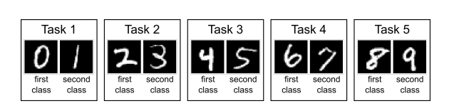
The split-MNIST protocol read through the three scenarios.
- Task-IL. $t$ given, so each task is a binary classifier $f_t:\c{X}\to\c{Y}_t$; for $t=3$ the model only decides between $4$ and $5$.
- Domain-IL. $t$ not given; all tasks relabeled into $\bar\c{Y}=\crbr{a,b}$ via $r_t(2t-2)=a,\ r_t(2t-1)=b$. The model answers “first or second digit of its pair?” so $0,2,4,6,8\mapsto a$ and $1,3,5,7,9\mapsto b$.
- Class-IL. $t$ not given; predict the actual digit $f:\c{X}\to\crbr{0,\dots,9}$, discriminating all ten classes with no task oracle.
The choice of setup dictates the success or failure of a method: parameter isolation works well for Task-IL but fails fundamentally for Class-IL. Modern work generalizes these into general and online continual learning, where data streams in a single epoch with no offline boundaries.3,4 The mitigation families that respond to these setups are the next entry.
1 Thrun & Mitchell 1995; Pan & Yang, “A survey on transfer learning,” IEEE TKDE 2009. 2 Liu & Chen, Lifelong Machine Learning, Morgan & Claypool 2018. 3 van de Ven & Tolias, “Three scenarios for continual learning,” arXiv:1904.07734; De Lange et al., IEEE TPAMI 2022. 4 Buzzega et al., “Dark experience for general continual learning,” arXiv:2004.07211; Bidaki et al., “Online continual learning: a systematic review,” arXiv:2501.04897. — next: forgetting and the mitigation families; the diffusion analogue of these three scenarios is here.
Continual learning for generative models: open questions
These notes are a working survey of continual learning, taken from the classical discriminative setting through to its diffusion-model form. I am writing them out one topic at a time. The recurring tension is always the same — stability versus plasticity — but where that tension lives changes completely once the object being learned is a generator rather than a classifier. The single question I keep returning to:
How much does the problem really change when task boundaries change continually, and what
is the right formal object to protect when the model is a score field rather than a
decision boundary?
The entries below build up the answer. The first five are classical continual learning; the rest are the diffusion-specific reformulation and its appendices.
Classical continual learning
- Formalisms and desiderata — what we are actually asking the learner to do, and the performance matrix.
- Definitions of tasks — Task-, Domain-, and Class-incremental learning.
- Forgetting and elastic weight consolidation — the three mitigation families and the Bayesian derivation of EWC.
- Replay and iCaRL — exemplar memory, nearest-mean classification, and generative rehearsal.
Diffusion models
- Problem statements — the diffusion analogues of the three scenarios.
- Choice of family — a controlled synthetic shift on a Gaussian mixture.
- Metrics — why a single scalar is never enough.
- Algorithms — replay, generative replay, distillation.
- Weight regularization — L2, EWC, and rank-1 Fisher in diffusion models.
- Function-space consolidation — PEFT, LoRA, masks, concept structure.
Appendices
- DDPM — the model, a 1-D Gaussian worked example, guidance (and the continuous-time view in Langevin dynamics).
- McCloskey–Cohen — the 1989 simulation that named the problem.
A few questions I cannot yet answer and want to keep in view: how badly do these problems degrade when task boundaries are not given at all (task-free streams); whether there is a principled multi-objective evaluation theory for continual diffusion, or whether the subject must stay irreducibly vector-valued; and what the correct mathematical notion of “not damaging the pretrained prior” even is. These thread through the later entries.
Formalisms and desiderata
Continual learning studies how a learner should update under non-stationary data streams without repeatedly retraining from scratch and without unacceptable degradation on previously relevant competencies. That is a starting definition; almost every word in it is still undefined. Here I want to pin down the desiderata, then the standard way the field actually summarizes a run — the performance matrix — and ask whether the same summaries survive the move to generative models.
§1. Short history
Modern continual learning is usually traced to two older threads. First, McCloskey and Cohen's 1989 paired-associate experiment, in which a network asked to learn an A–C mapping on top of an A–B mapping forgot the first almost completely — the simulation that named catastrophic interference (its full setup is its own entry). Second, Thrun's mid-1990s lifelong-learning program, asking how experience on earlier problems can bias later ones across related classification tasks.1 Work since then sharpened the problem around catastrophic forgetting in neural networks, clarified benchmark scenarios (task-, domain-, class-incremental, the subject of the next entry), and extended the setting to task-free and online streams where boundaries are not given.2
Definition (classical task-based continual learning). Let $\c{X}$ be an
input space and $\c{Y}$ a target space. A continual learning problem is a sequence of tasks
$\c{T}=(\c{T}_1,\dots,\c{T}_N)$, where each task $\c{T}_t$ is a stationary distribution
$P_t$ on $\c{X}\times\c{Y}$. At stage $t$ the learner sees only a finite dataset
$\c{D}_t\sim P_t$ and must update its parameters sequentially so that performance on
previously encountered tasks does not degrade substantially as new tasks arrive.
This discrete-task picture — well-separated stationary blocks, often with known task boundaries — dominated the pre-2020 literature. The major shift came with task-free and online continual learning, where one is not told when the task changes. Since 2025, in foundation-model settings, the meaning of “task” has broadened further.2,3
§2. What is a good desideratum?
There is no single task-independent desideratum that is universally correct. A good one should be deployment-faithful. A minimal set:
- Retention: preserving performance on previously relevant competencies.
- Plasticity and transfer: rapidly acquiring new competencies while enabling positive forward or backward transfer when tasks are related.
- Observability consistency: not relying on task identifiers or oracle task boundaries unless such information is genuinely available at deployment.
- Efficiency: respecting memory, compute, and possibly privacy constraints.
For foundation models one should additionally track preservation of broad pretrained knowledge, instruction-following, and safety/alignment. Two failure modes specific to LLMs are worth naming: cross-stage forgetting, where pre-training, SFT, and preference optimization interact destructively; and pseudo-forgetting, where the model retains a latent capability but fails to activate it under the current prompting distribution — instruction-following misalignment rather than true overwriting.4
§3. The performance matrix
Training optimizes a loss, but continual learning is summarized by a performance
matrix. Given a stream $\crbr{\c{T}_t}_{t=1}^T$, let
$\theta_t := U_t(\theta_{t-1},\c{T}_t)$ be the model after updating on task $\c{T}_t$, and
let
$$ a_{t,k} := M_k(\theta_t) $$
denote performance on task $k$ after finishing training on task $t$ (accuracy, IoU, BLEU,
or any task-specific metric). The diagonal $a_{t,t}$ is performance immediately after a
task is learned; entries with $k
The matrix supports four standard summaries.
$$ \mathrm{ACC}_t = \frac1t\sum_{k=1}^t a_{t,k}
\qquad\text{(average accuracy so far)} $$
$$ \mathrm{BWT}_t = \frac1{t-1}\sum_{k=1}^{t-1}\smbr{a_{t,k}-a_{k,k}}
\qquad\text{(backward transfer)} $$
$$ \mathrm{FM}_t = \frac1{t-1}\sum_{k=1}^{t-1}\smbr{\max_{1\le\ell\le t-1}a_{\ell,k}-a_{t,k}}
\qquad\text{(forgetting)} $$
$$ \mathrm{FWT}_t = \frac1{t-1}\sum_{k=2}^{t}\smbr{a_{k-1,k}-b_k}
\qquad\text{(forward transfer)} $$
Negative BWT indicates forgetting; positive BWT means later tasks improved earlier ones. FM is finer: it compares the current score to the best score ever achieved on each old task, so it is a direct loss-of-capability statistic. FWT compares pre-training-on-task-$k$ performance $a_{k-1,k}$ to a from-scratch baseline $b_k$. One may also report $a_{t,t}$ alone as a plasticity score, but these four are the main matrix-based summaries.
§4. Do the same metrics work for generative models?
Not cleanly. For an LLM the per-task score is already a vector, $$ M_k(\theta_t) := \smbr{M_k^{\mathrm{task}}(\theta_t),\, M_k^{\mathrm{instr}}(\theta_t),\, M_k^{\mathrm{safety}}(\theta_t),\,\dots} $$ TRACE makes this explicit: alongside traditional continual-learning metrics it adds a General Ability Delta, an Instruction-Following Delta, and a Safety Delta, each an average post-training shift relative to the initial aligned model.5 The same vector-valued character returns, more severely, for diffusion models — visual plausibility, prompt following, old-task retention, and compositional reuse can each fail independently, which is the whole point of the metrics entry.
1 Thrun, “Lifelong learning algorithms,” in Learning to Learn, Springer 1998; Thrun & Mitchell, Lifelong Robot Learning, 1995. 2 McCloskey & Cohen, Psych. Learn. Motiv. 1989; van de Ven & Tolias, “Three scenarios for continual learning,” arXiv:1904.07734; Aljundi et al., “Task-free continual learning,” CVPR 2019; De Lange et al., IEEE TPAMI 2022. 3 Bell et al., “The future of continual learning in the era of foundation models,” arXiv:2506.03320; Guo et al., “A comprehensive survey on continual learning in generative models,” arXiv:2506.13045. 4 Sun et al., “Unveiling and addressing pseudo forgetting in LLMs,” Findings of ACL 2025. 5 Wang et al., “TRACE: a comprehensive benchmark for continual learning in LLMs,” arXiv:2310.06762. — next: the three discriminative scenarios, definitions of tasks.